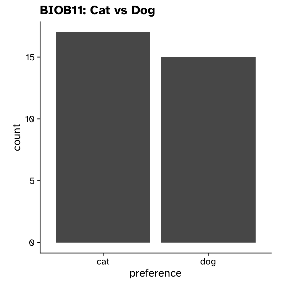
# A tibble: 32 × 1
   preference
   <chr>
 1 cat
 2 dog
 3 dog
 4 dog
 5 dog
 6 cat
 7 dog
 8 dog
 9 cat
10 dog
# ℹ 22 more rowsTest of and associations between categorical variables
Lecture 6
2025-04-02
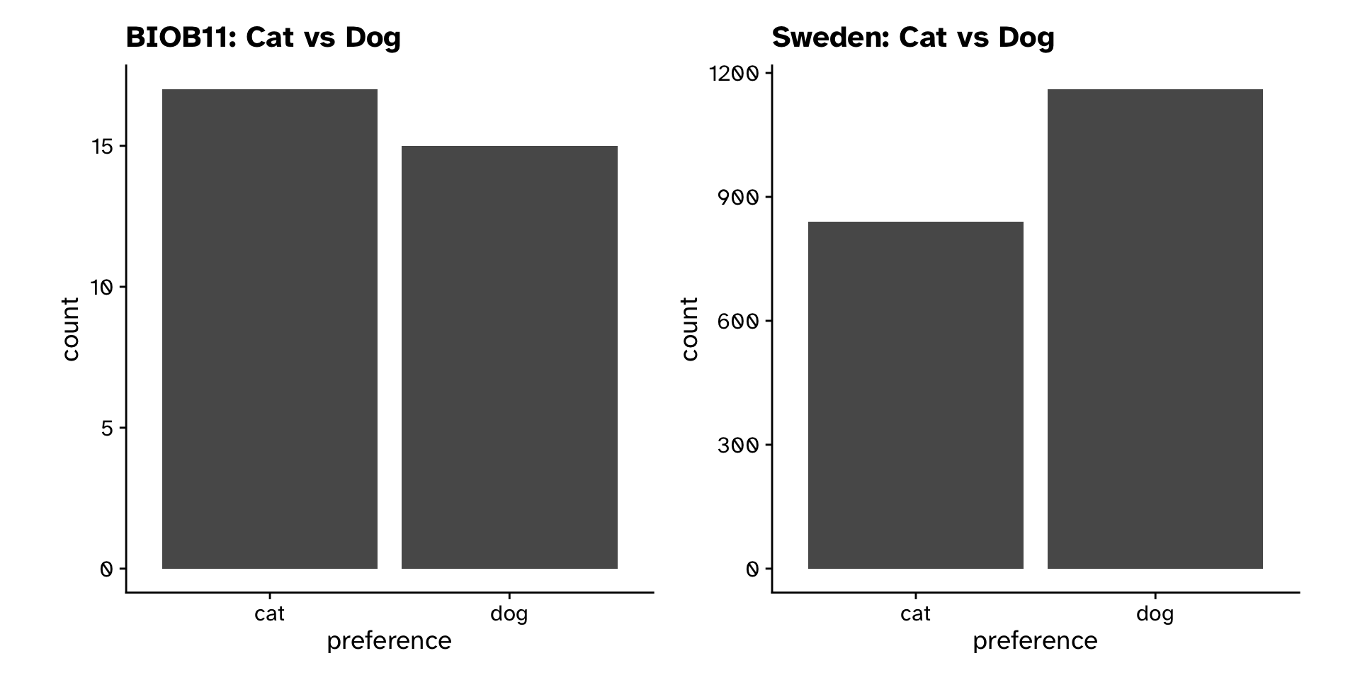
Tests of proportion
Could a proportion have been observed under a null hypothesis?
Tests of proportion
Could a proportion have been observed under a null hypothesis?
Tests of proportion
Could a proportion have been observed under a null hypothesis?
Tests of proportion
Could a proportion have been observed under a null hypothesis?
Tests of proportion
Could a proportion have been observed under a null hypothesis?
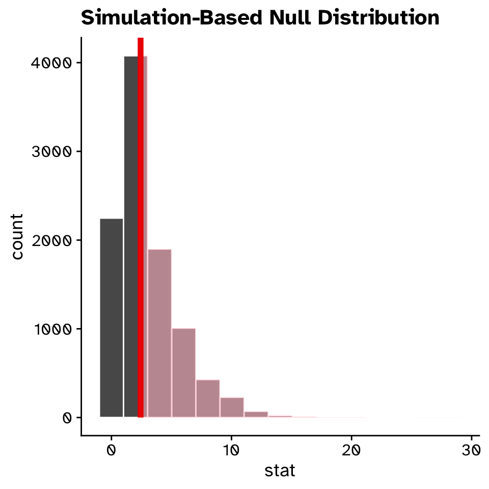
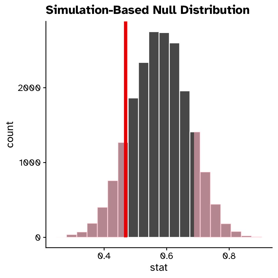
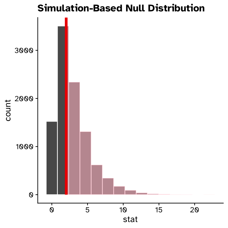
Visualise the null:
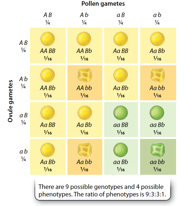
\(\chi^2\) Goodness of fit
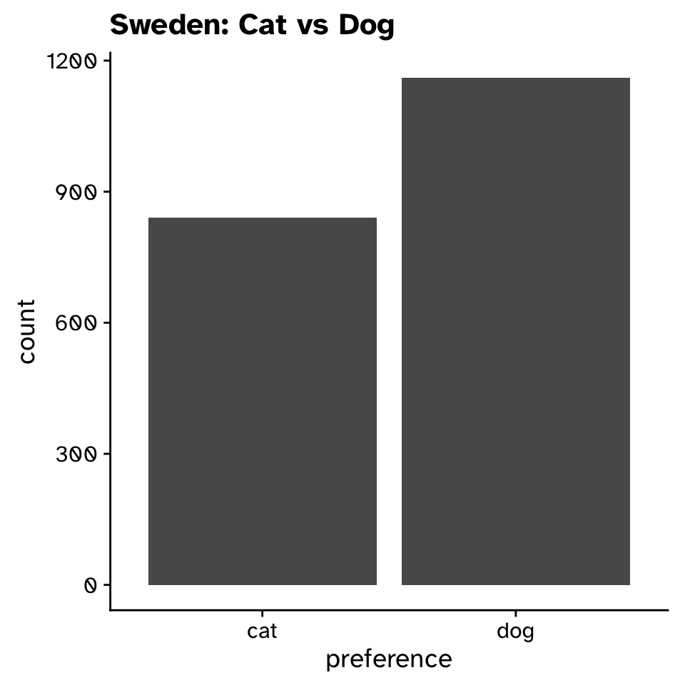
Does the observed data differ from an expected distribution?
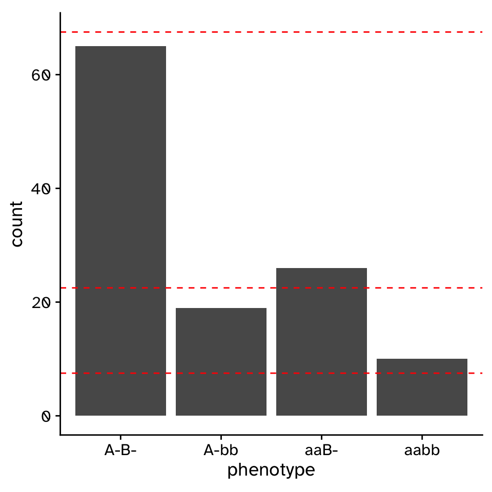
\(\chi^2\) Goodness of fit
Does the observed data differ from an expected distribution?
\(\chi^2\) Goodness of fit
Does the observed data differ from an expected distribution?
\(\chi^2\) Test of independence
Are two categorical variables associated with each other?
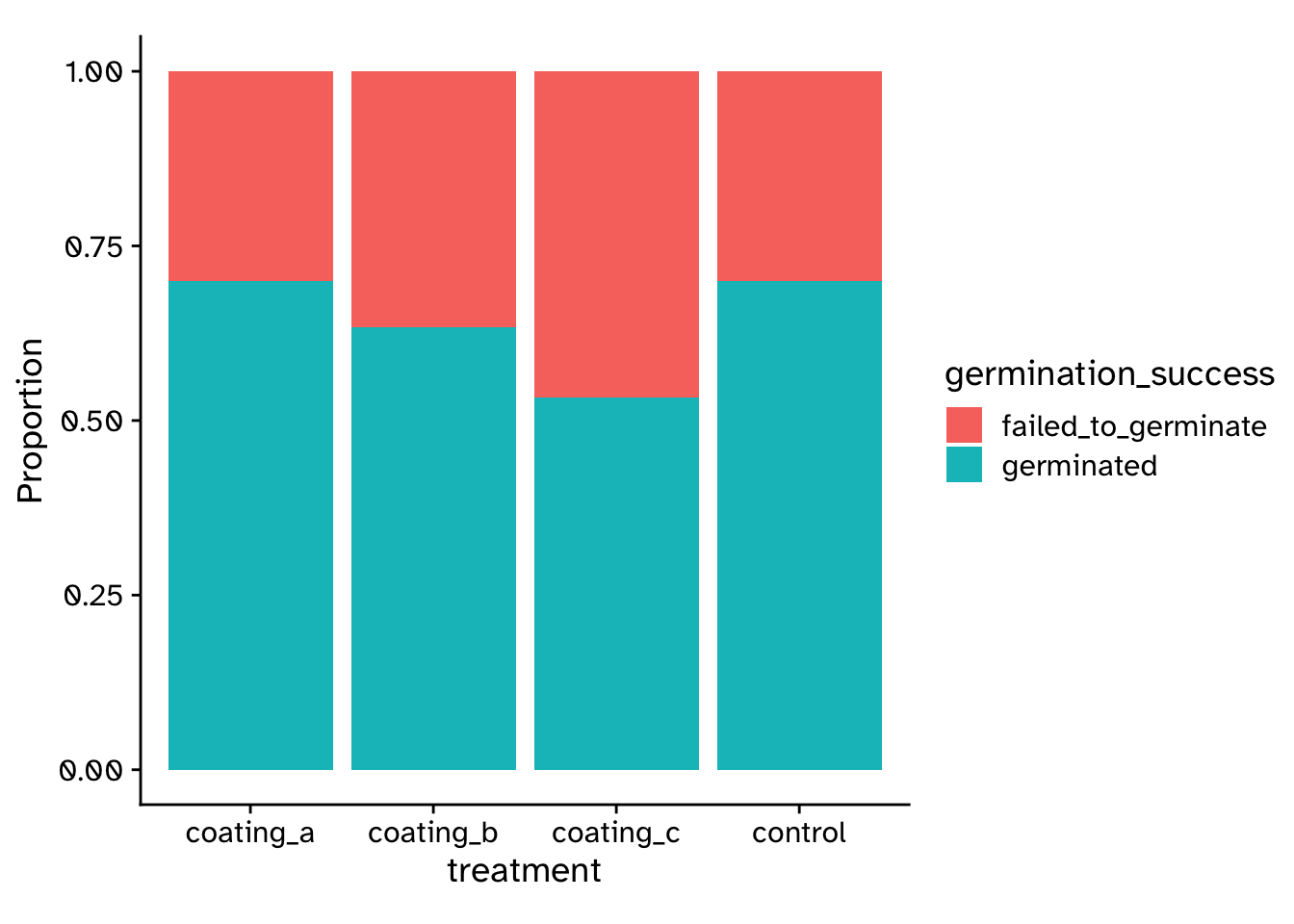
\(\chi^2\) Test of independence
Are two categorical variables associated with each other?