Regression modelling
Lecture 6
Wednesday 1st April, 2026
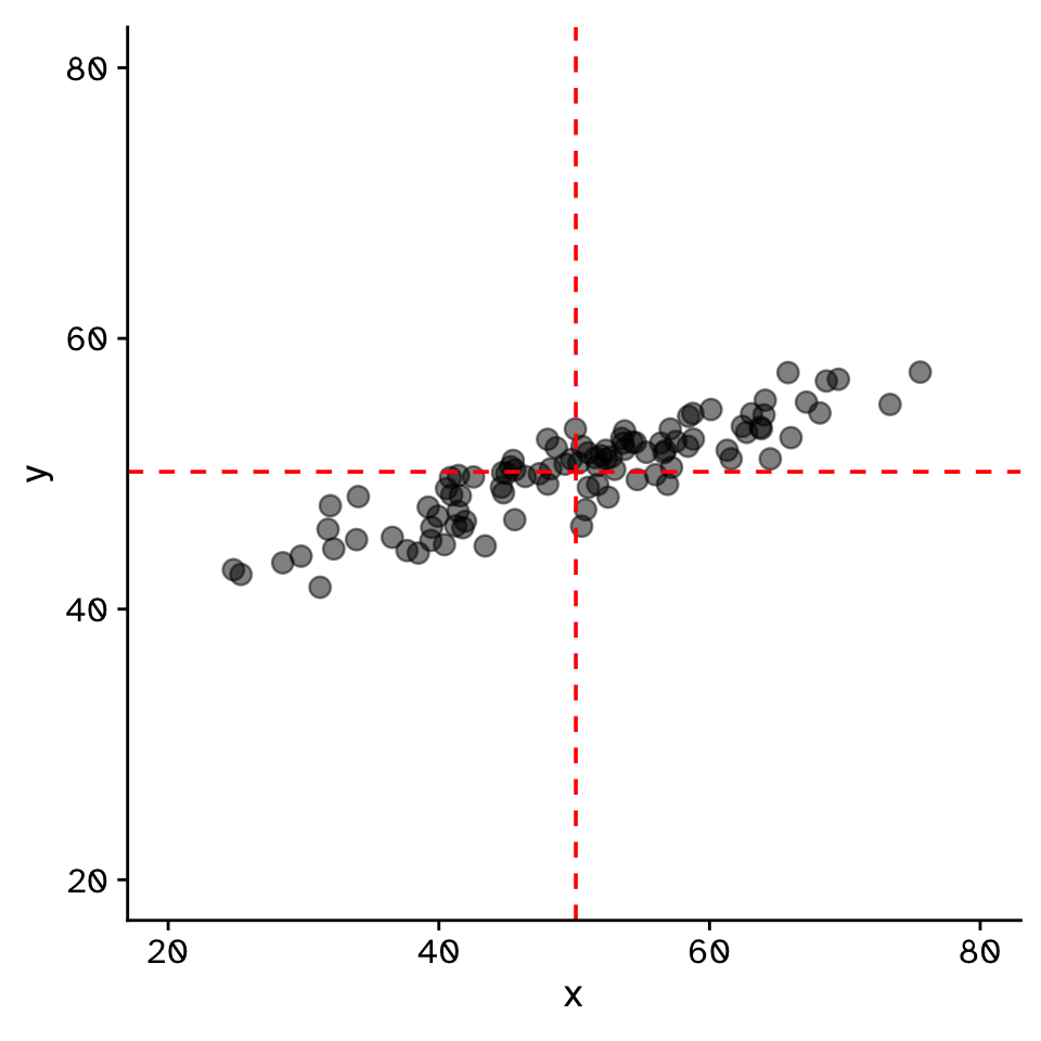
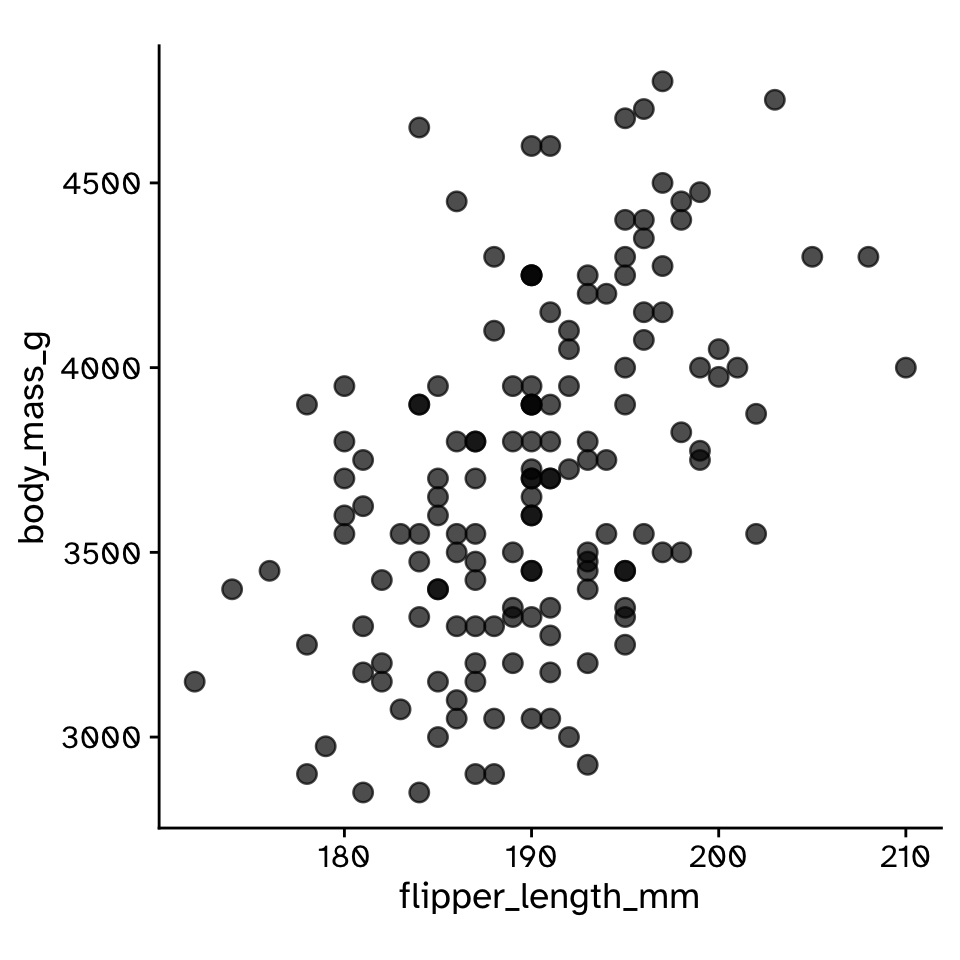
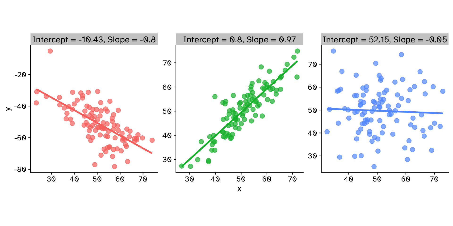
Correlation
Do two continuous variables covary?
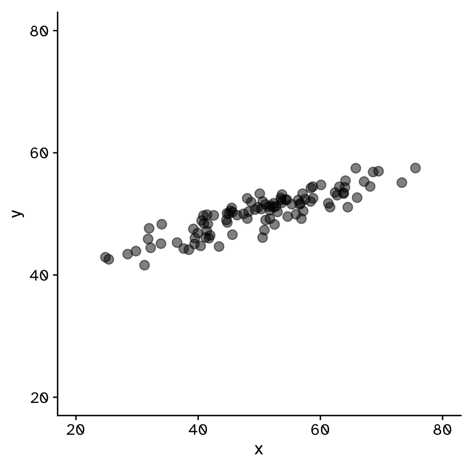
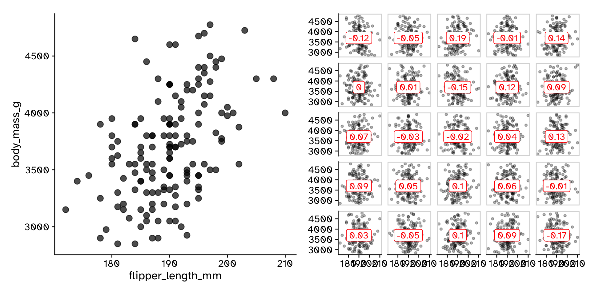
Correlation
Do two continuous variables covary?
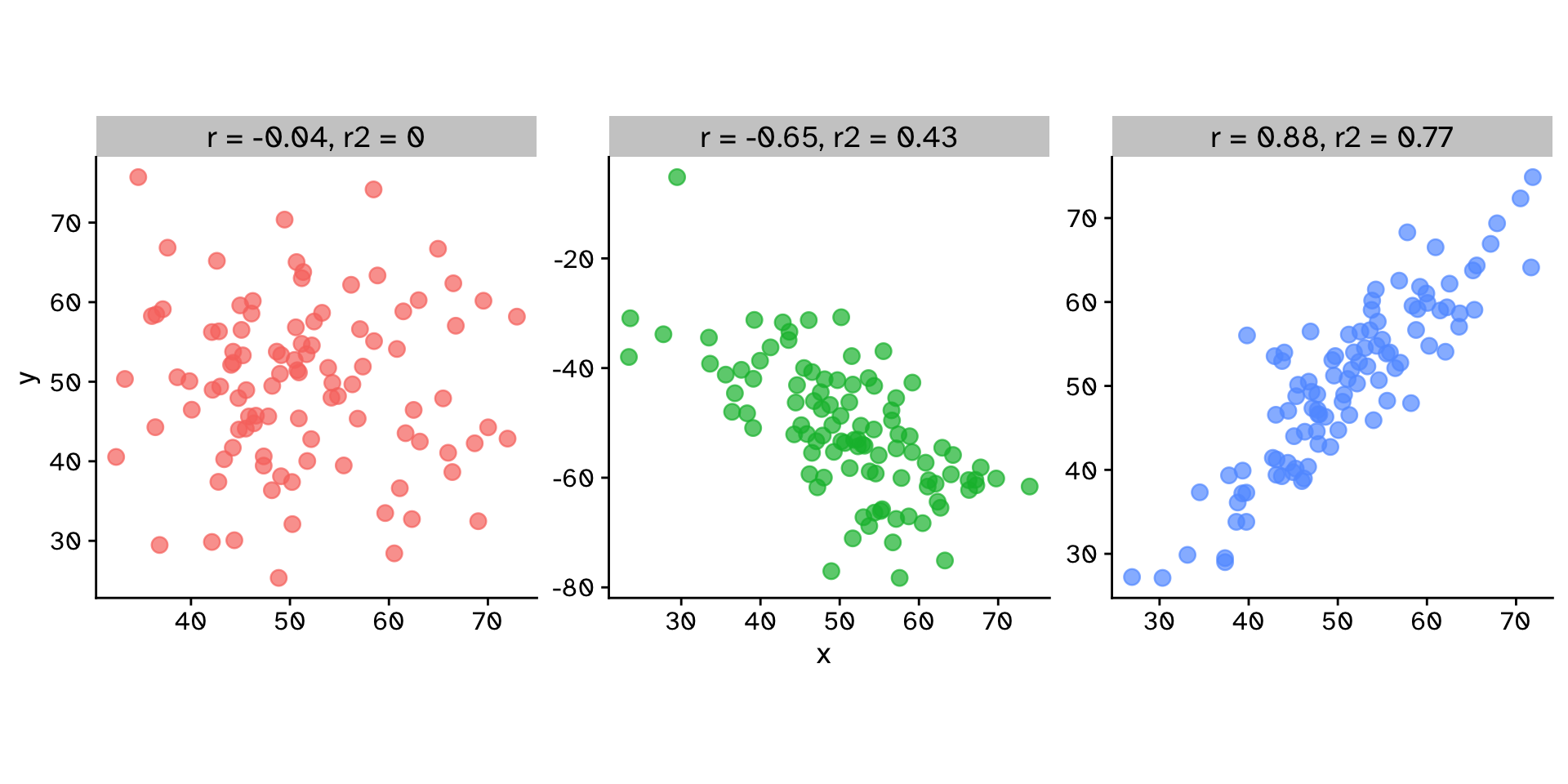
Correlation
Do two continuous variables covary?
Correlation
Do two continuous variables covary?
Correlation
Do two continuous variables covary?

Correlation
Do two continuous variables covary?
Correlation
Do two continuous variables covary?

Correlation
Confidence intervals
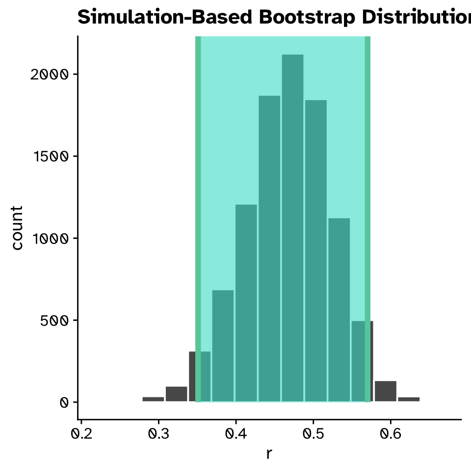
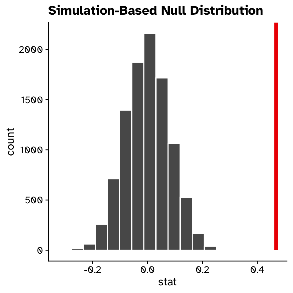
Correlation
Hypothesis test
- How could we generate a null distribution?
Correlation
Hypothesis test
Correlation
Hypothesis test
Linear Regression
How does variable Y depend on variable X
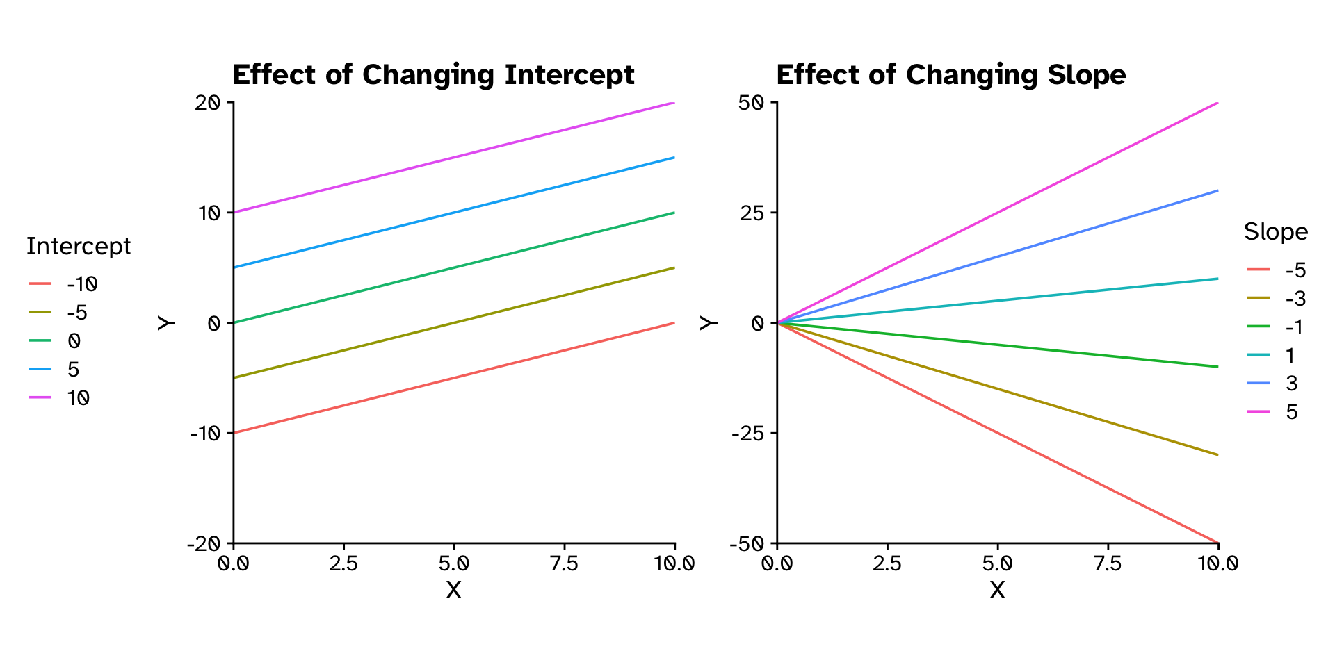
Linear Regression
How does variable Y depend on variable X
Linear Regression
How does variable Y depend on variable X
- Example: For sexual selection to operate, an increase in mating success (number of mates) must result in an increase in reproductive success (number of offspring).
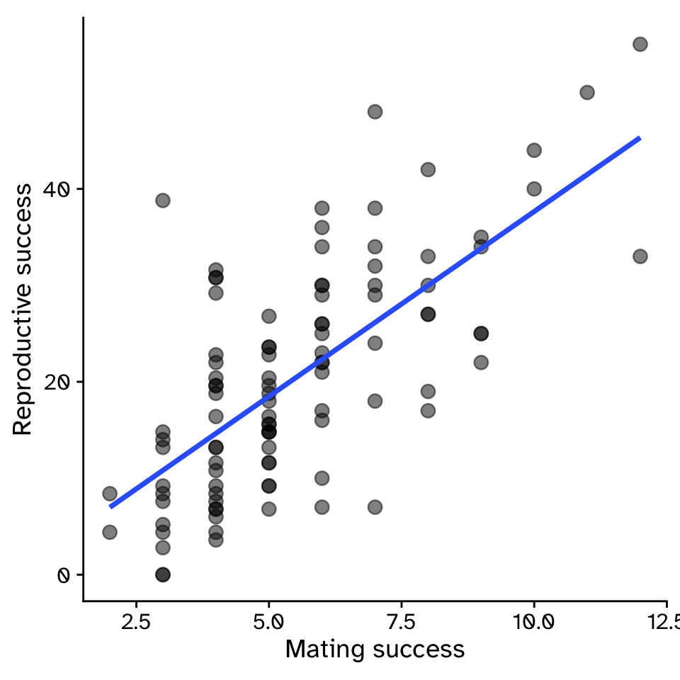
Linear Regression
How does variable Y depend on variable X
\[ y = \beta_1x+\beta_0 \]
\[ y = 3.83x-0.68 \]
- \(\beta_1\) = strength of sexual selection
- For each additional mate, an individual (on average) gains \(\beta_1\) additional offspring
- For 5 mates (\(x=5\)):
- \(y = 3.83\times5-0.68\)
- \(y = 18.47\)

Linear Regression
How does variable Y depend on variable X
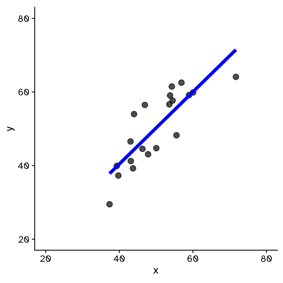
Linear Regression
How does variable Y depend on variable X
Linear Regression
How does variable Y depend on variable X

Linear Regression
How does variable Y depend on variable X
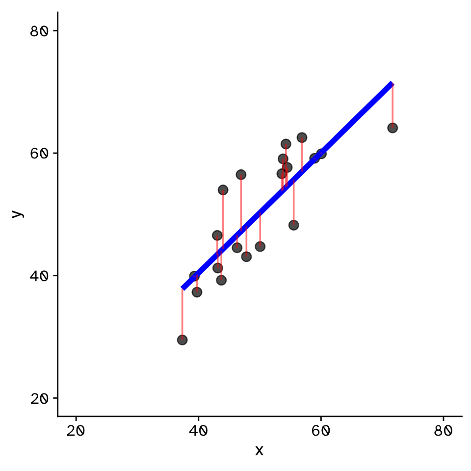
Linear Regression
- Fit by solving to minimise the sum of the squared residuals (SSR)
- Find \(\beta_1\) and \(\beta_0\) that minimise the SSR
- Called a “loss function”
Linear Regression
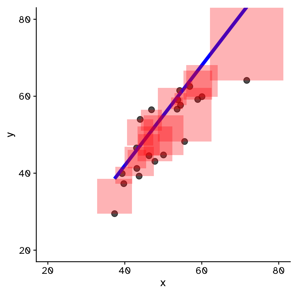
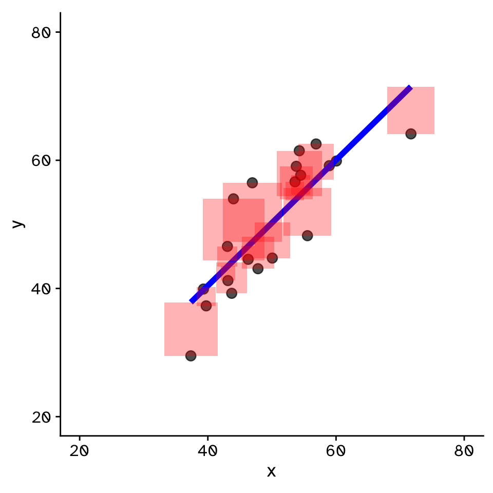
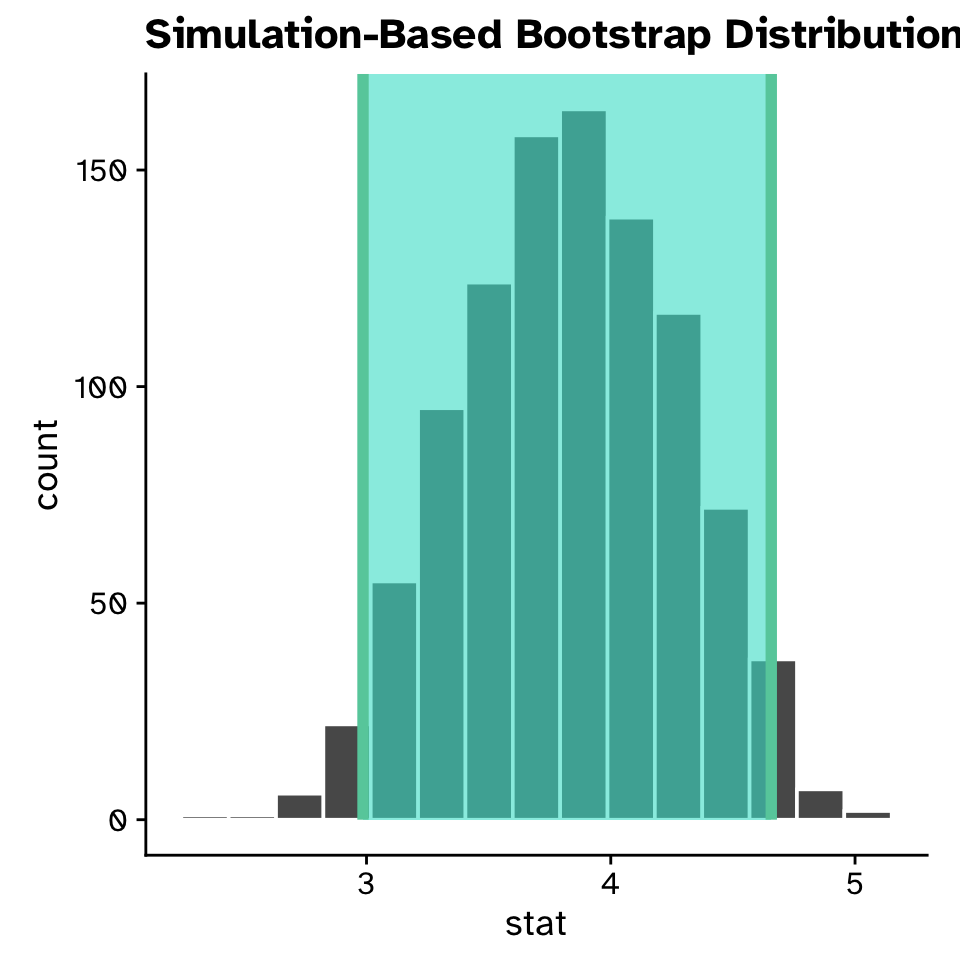
Confidence intervals for a slope

Linear Regression
Confidence intervals for a slope
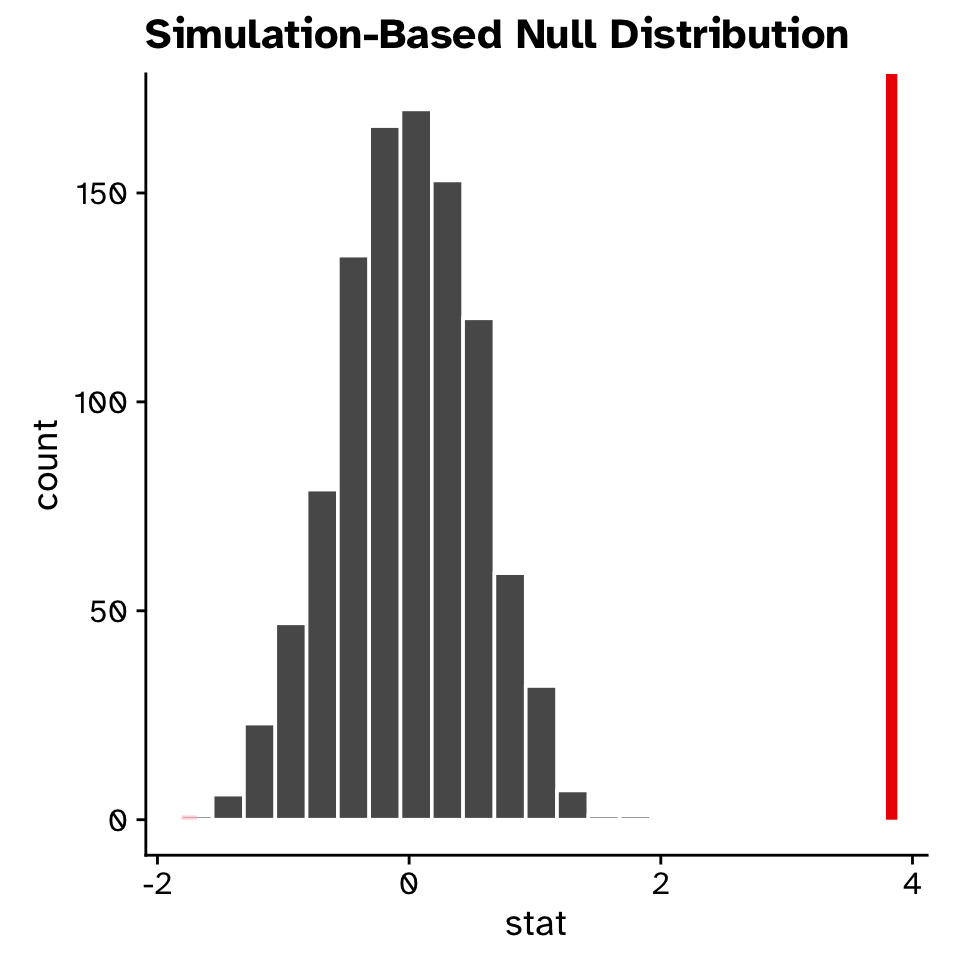
Linear Regression
Hypothesis test for a slope
Linear Regression
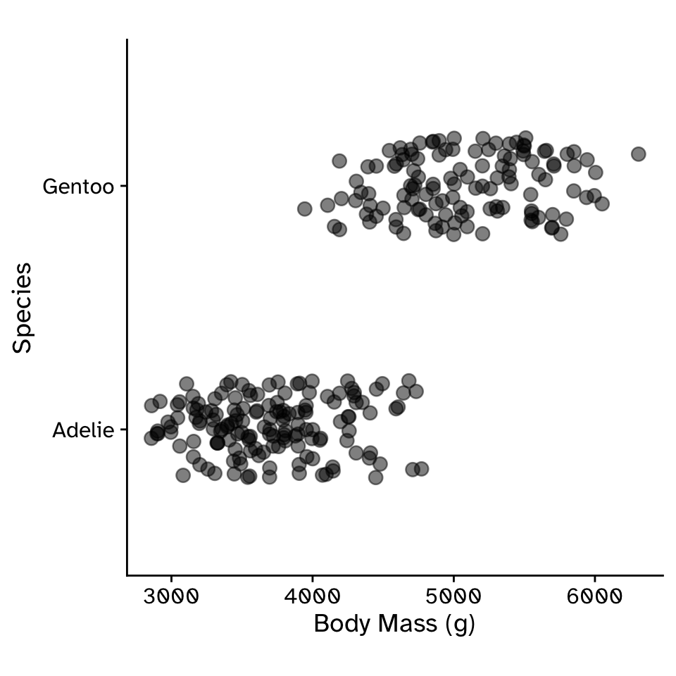
Multiple linear regression: intercept only model
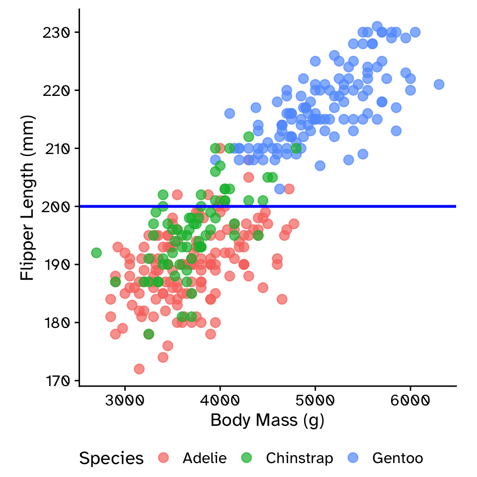
Linear Regression
Multiple linear regression: intercept and slope model
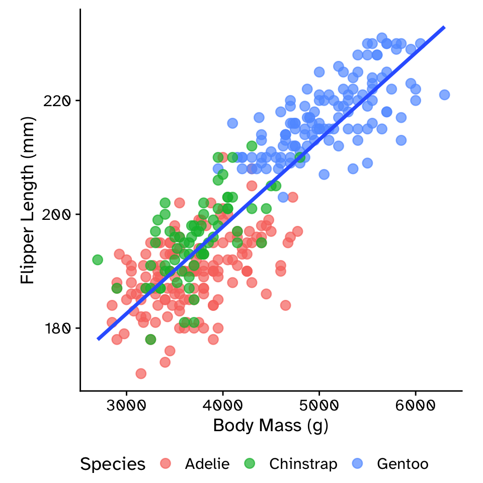
Linear Regression
Multiple linear regression: additive model with parallel slopes (ANCOVA)
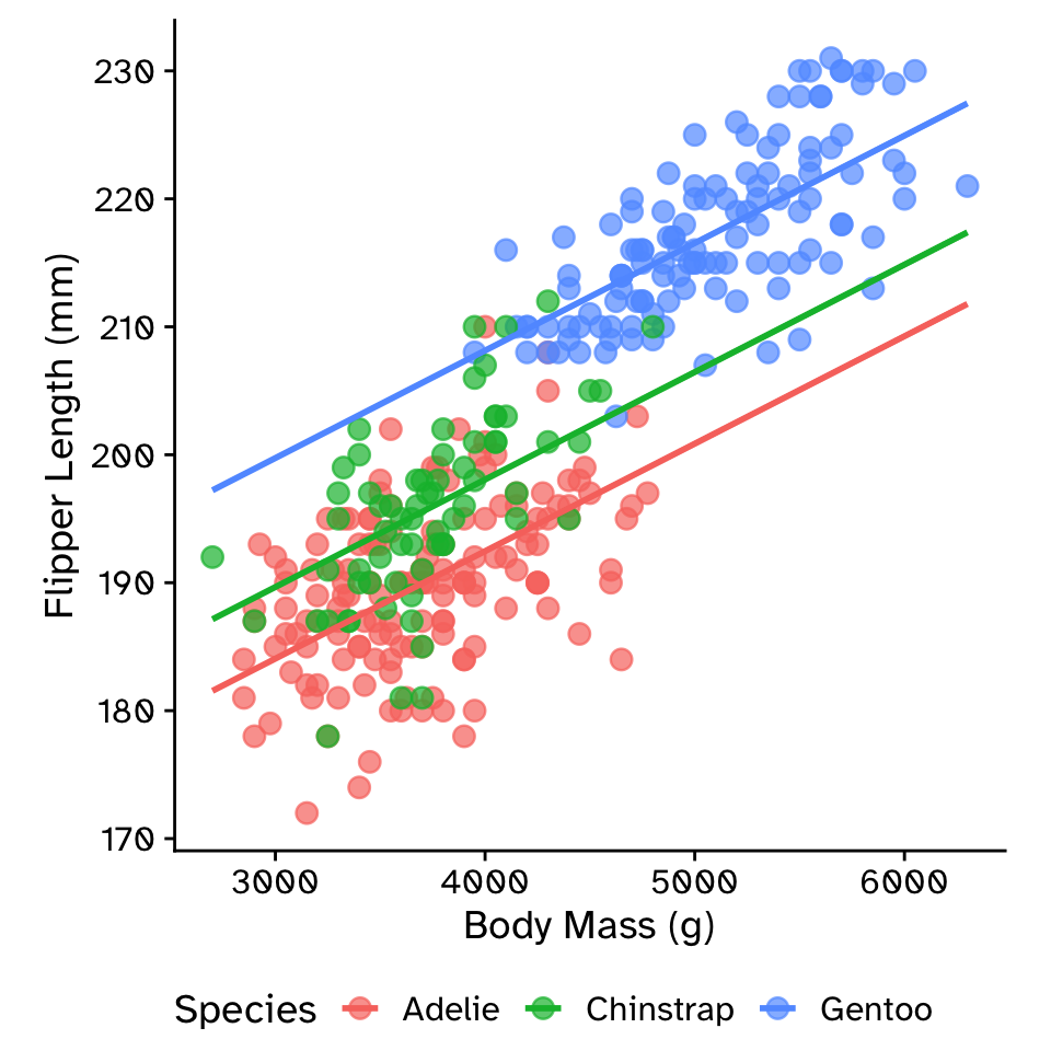
\[ \text{flipper_length_mm} = \beta_0+ \\ \beta_1 \times \text{body_mass_g}+ \\ \beta_2 \times \text{species} \]
Linear Regression
Multiple linear regression: interaction model
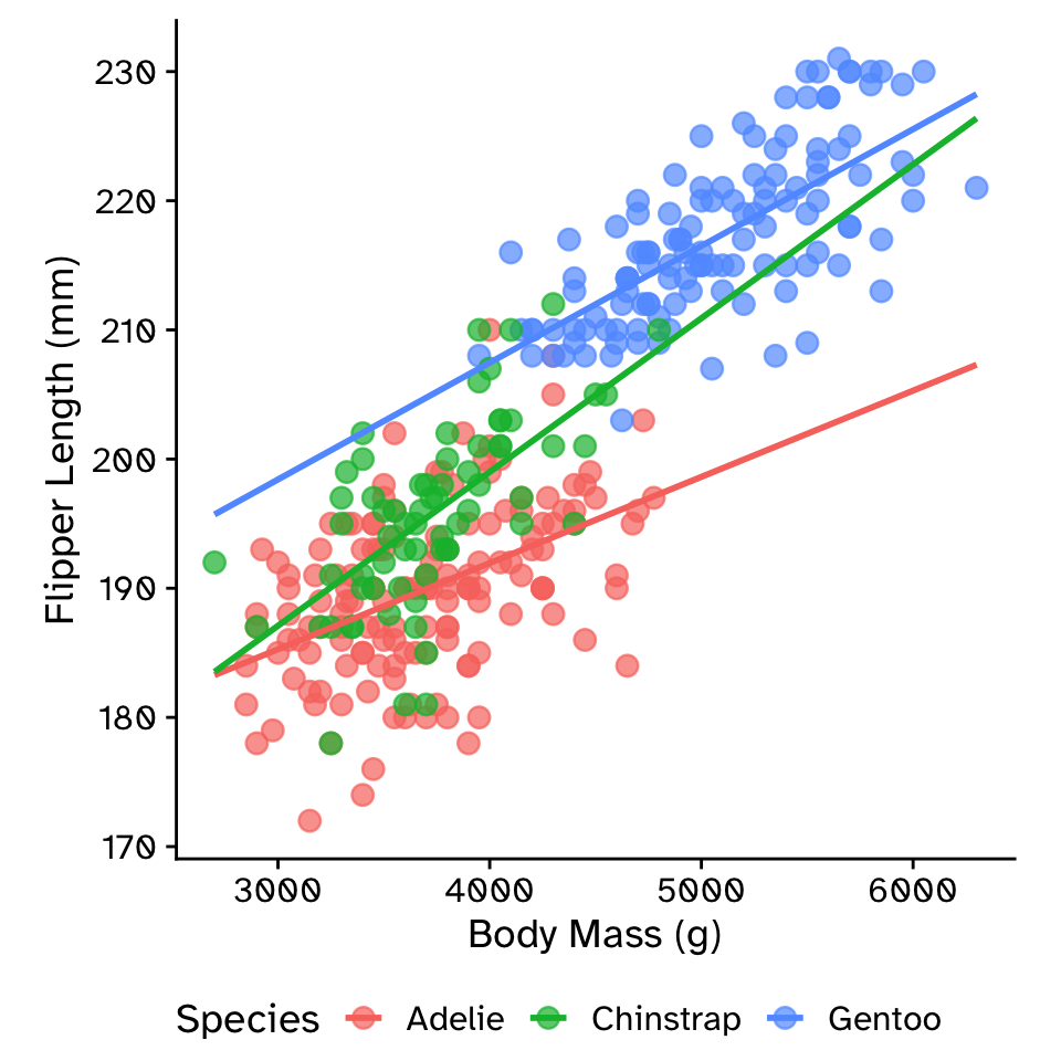
\[ \text{flipper_length_mm} = \beta_0 + \\ \beta_1 \times \text{body_mass_g} + \\ \beta_2 \times \text{species} + \\ \beta_3 \times \text{body_mass_g} \times \text{species} \]
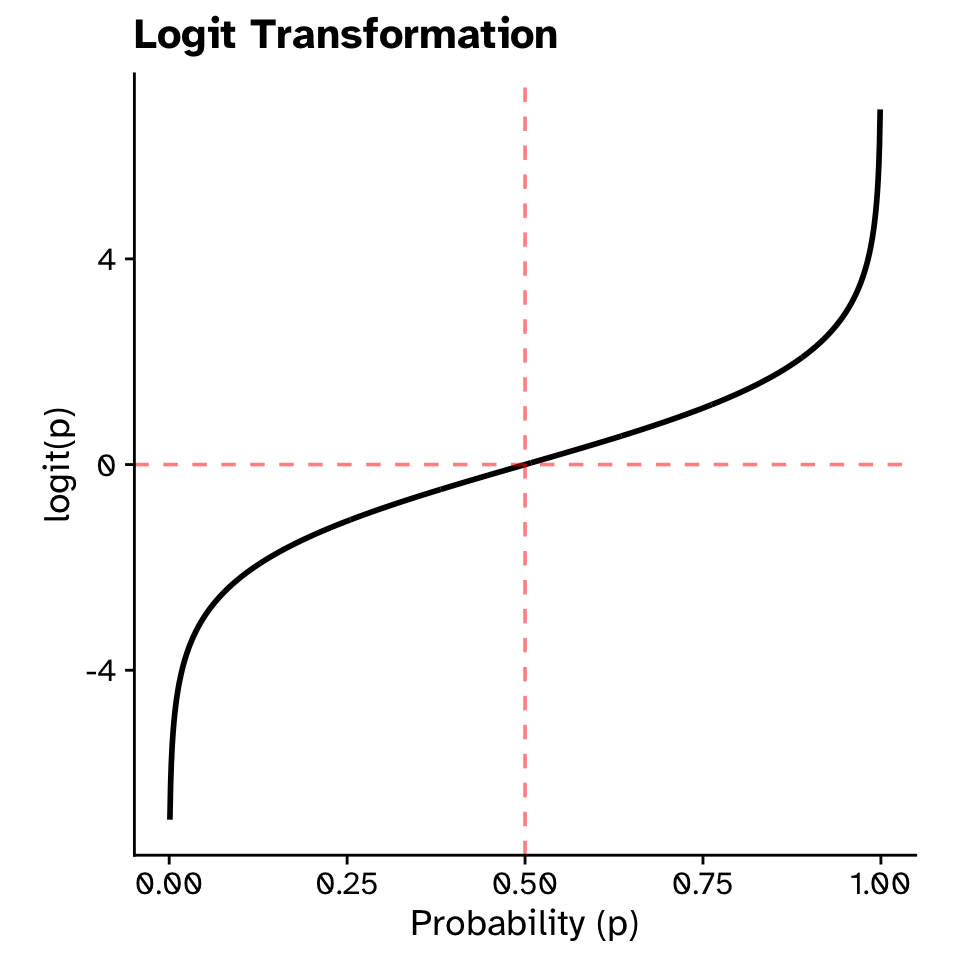
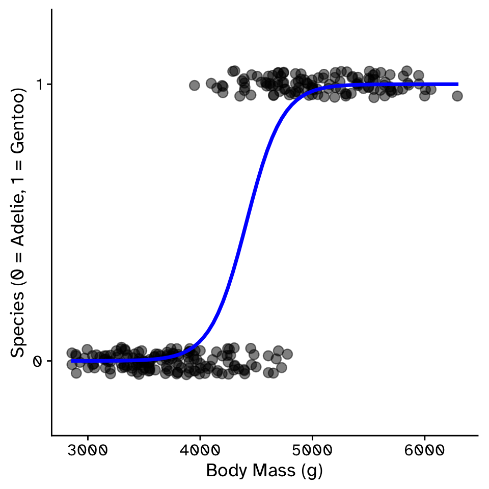
Logistic Regression
Predicting a binomial response with a quantitative variable
Logistic Regression
Logit transformation