Statistical inference with mathematical models
Lecture 7
Tuesday 7th April, 2026
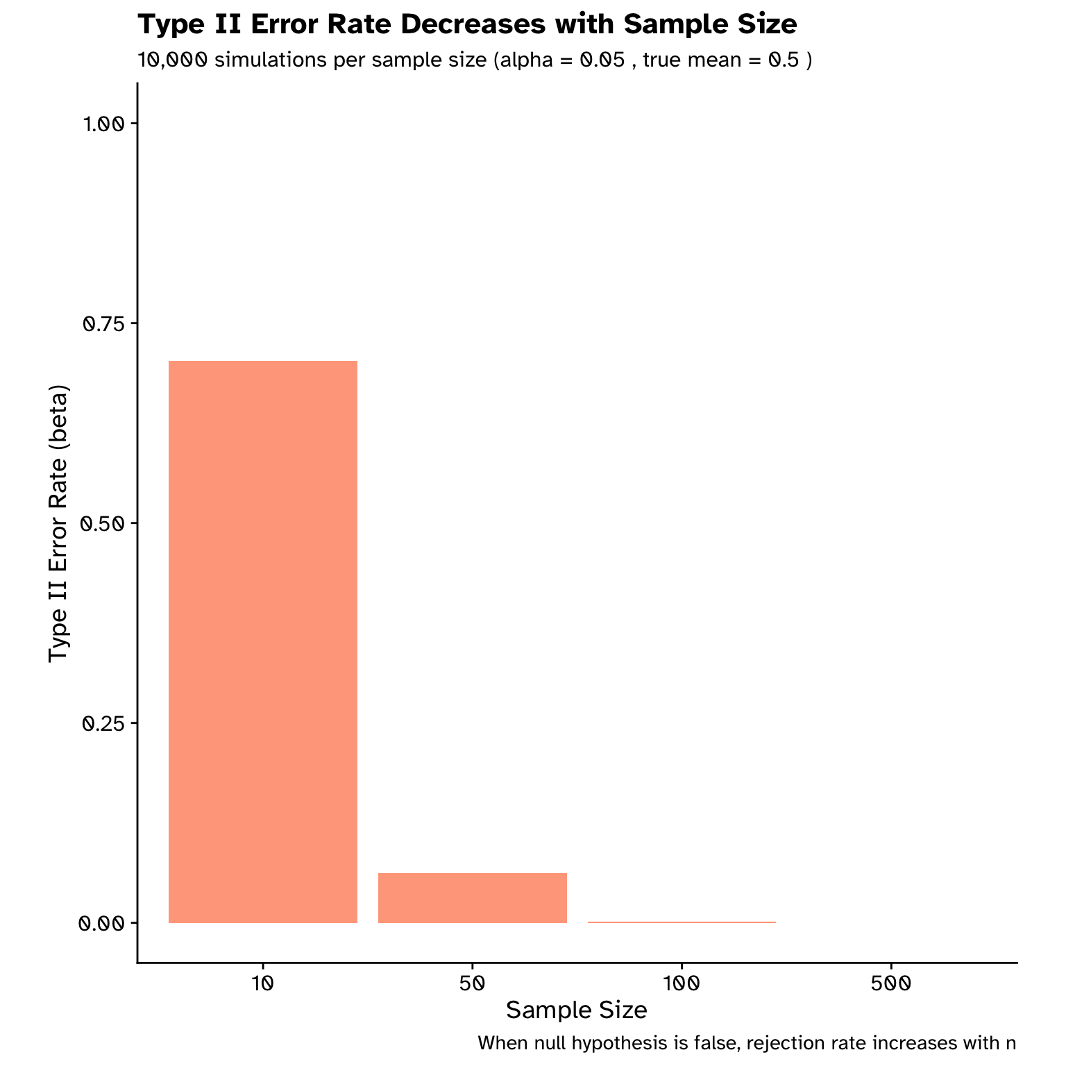
Making an error
Types of error (hypothesis testing)
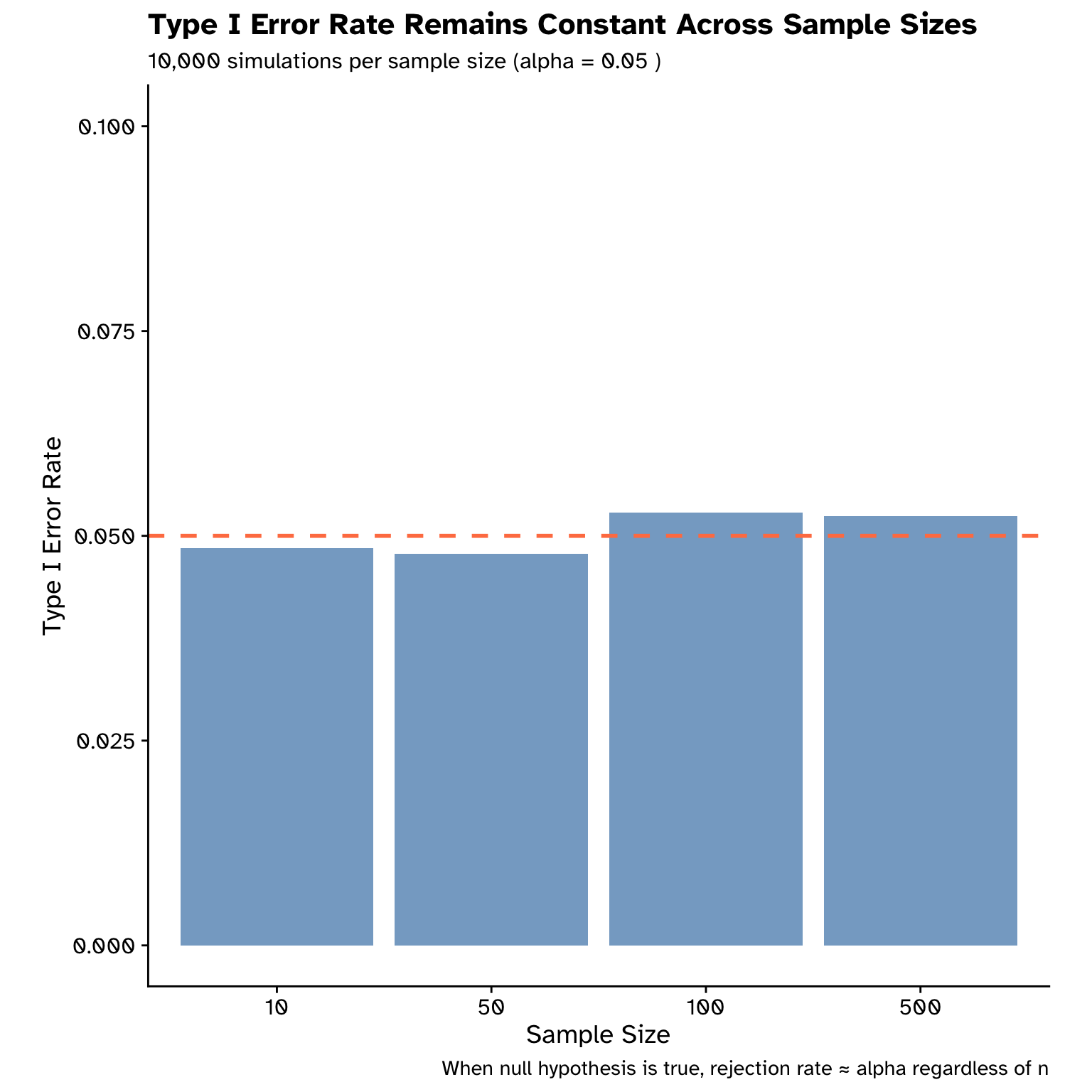
Making an error
Types of error (hypothesis testing)
Probability distributions
Bimodal distribution: flipping a coin
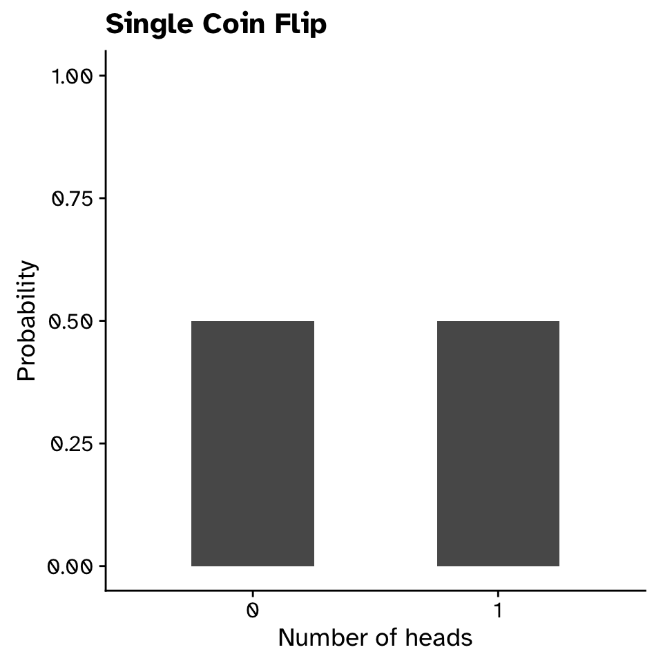
Probability distributions
Bimodal distribution: flipping a coin
Probability distributions
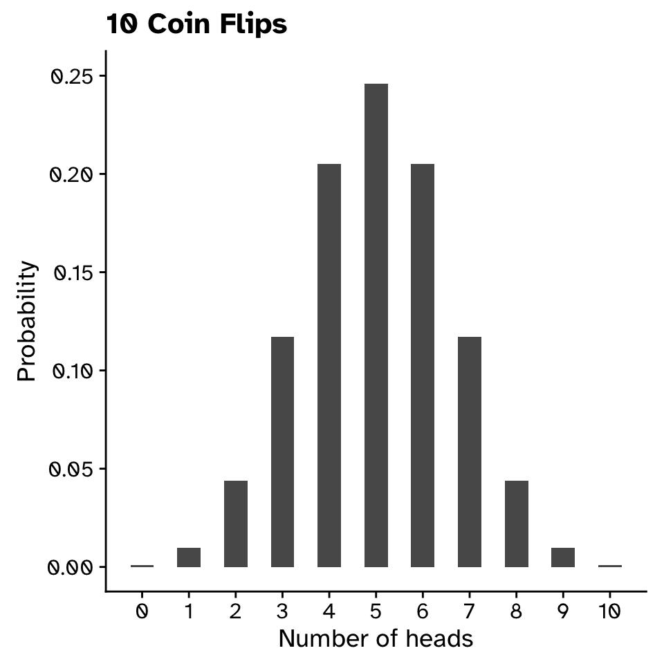
Bimodal distribution: flipping a coin

- \(P(X=5)=0.25\)
- \(P(4\le X\le6)=0.25+0.2+0.2\)
- \(P(X \ge 9) \approx 0.011\)
Probability distributions
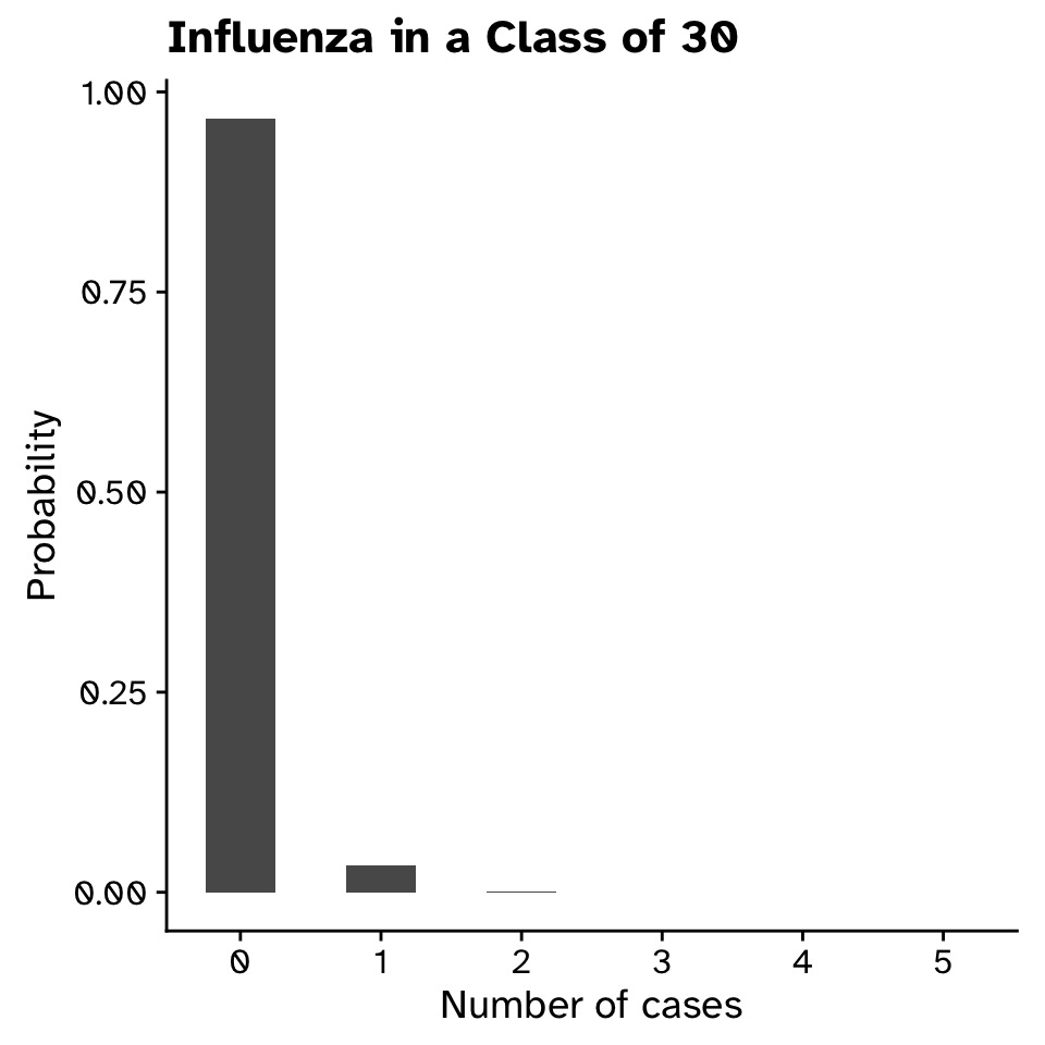
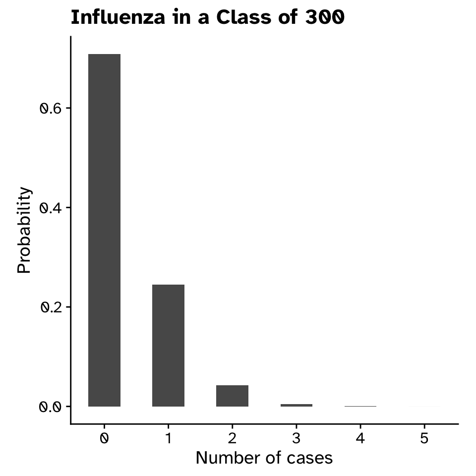
Bimodal distribution: Influenza
Probability distributions
Bimodal distribution: Influenza
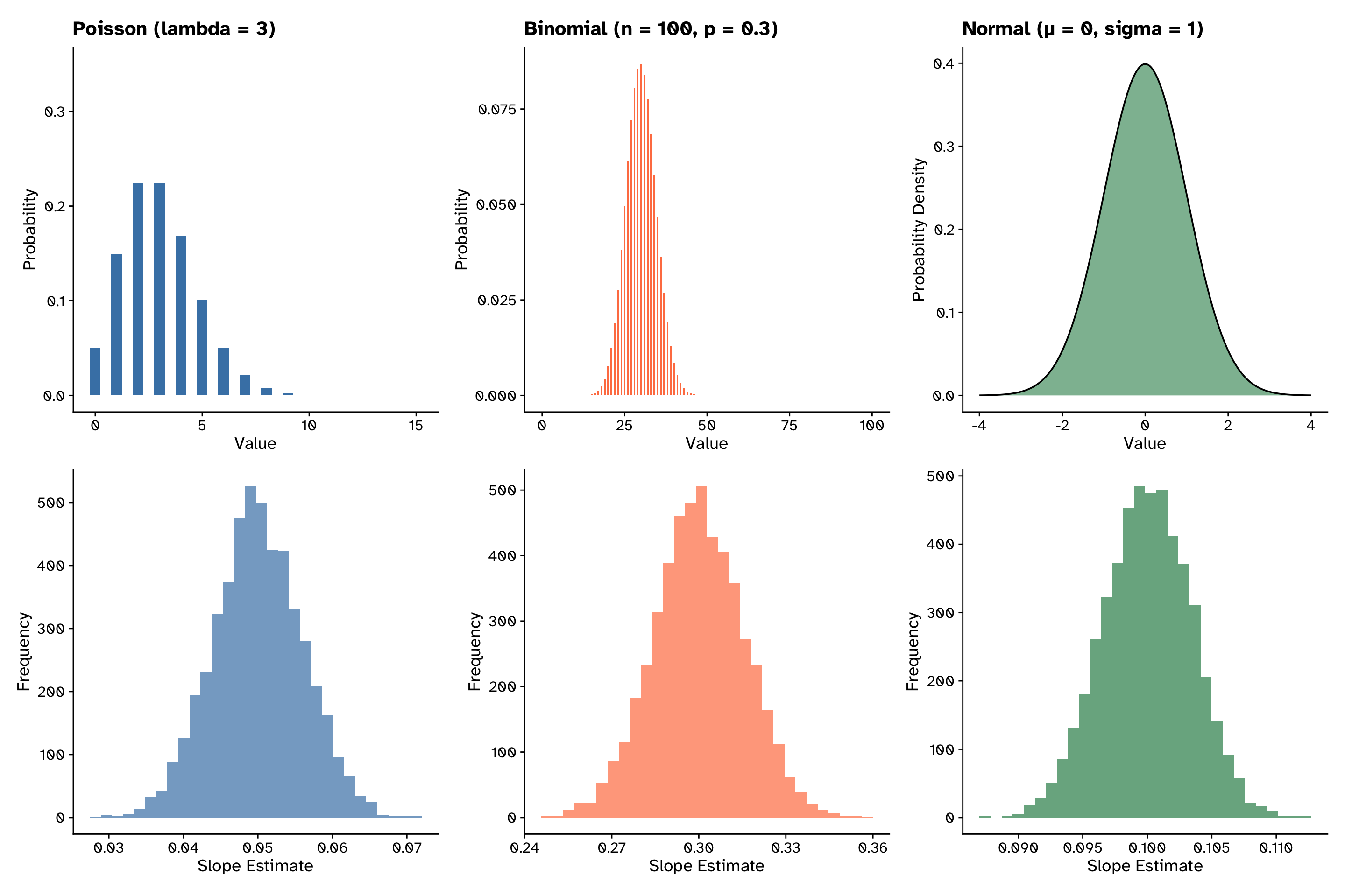
Probability distributions
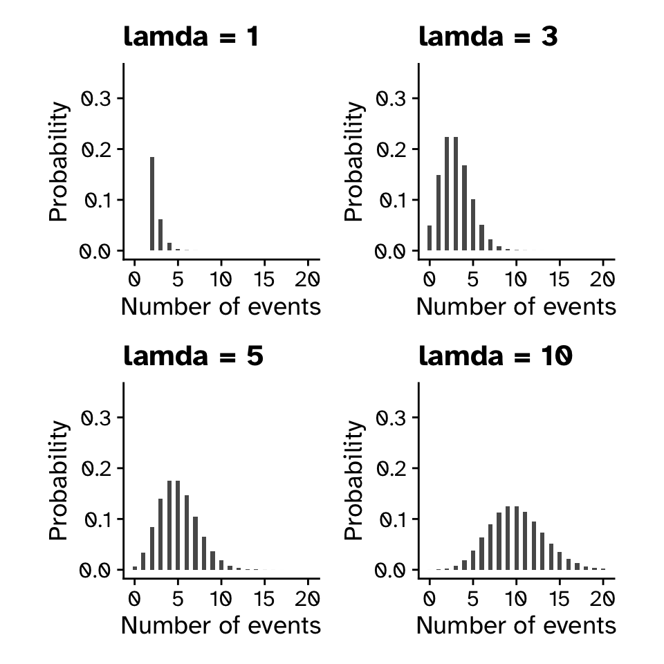
Poisson distribution
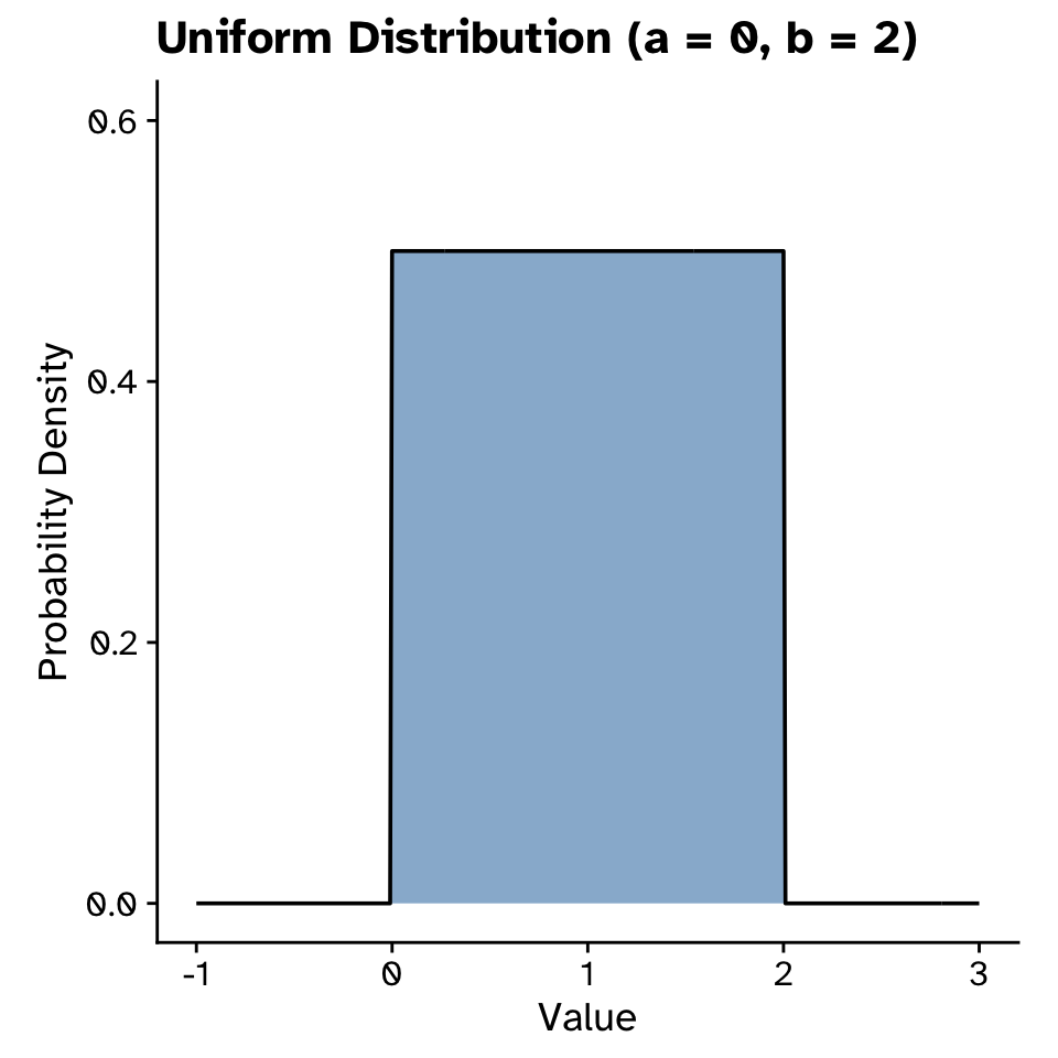
Probability distributions
Uniform distribution
- Not meaningful to ask probability of specific number
- Instead look at probability of intervals
Probability distributions
Normal distribution
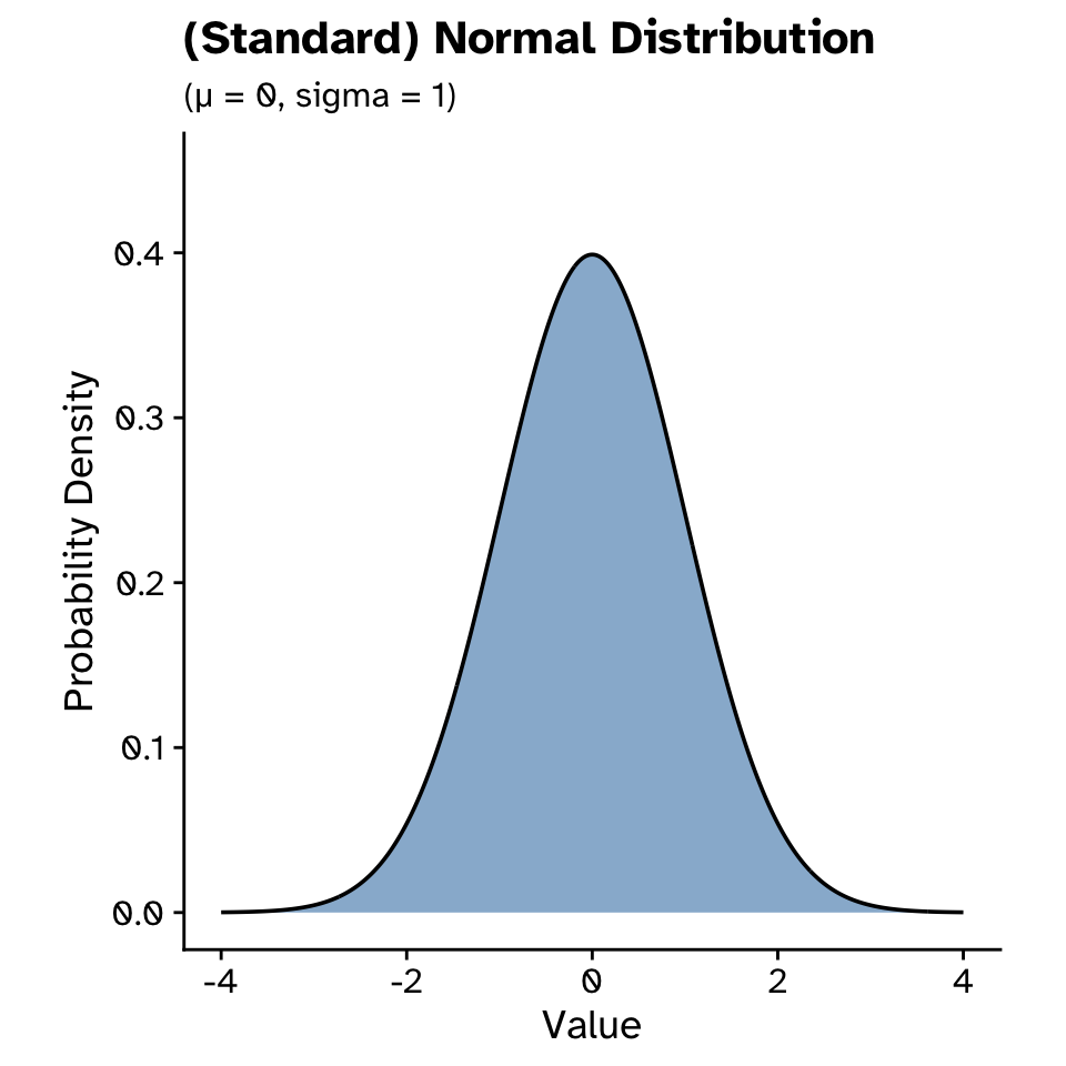
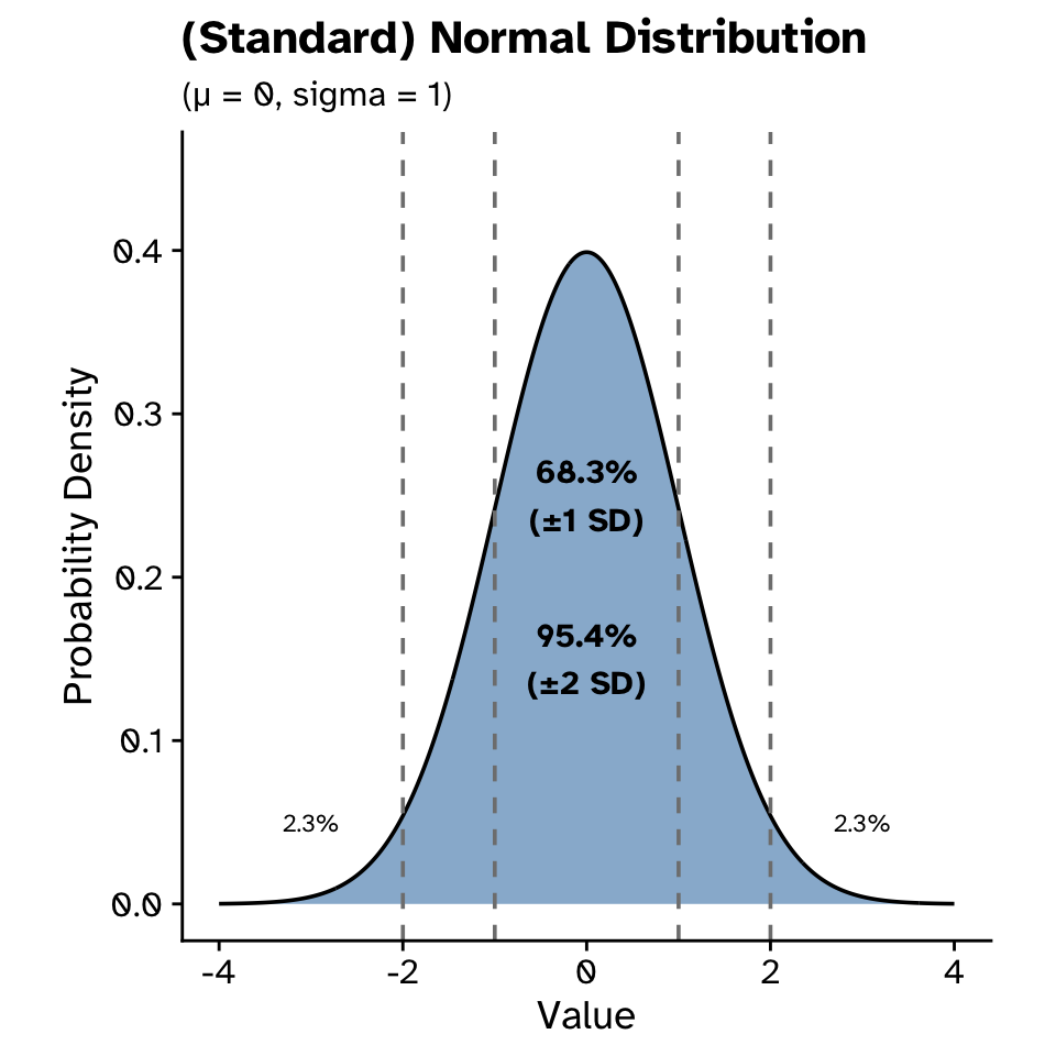
Probability distributions
Normal distribution
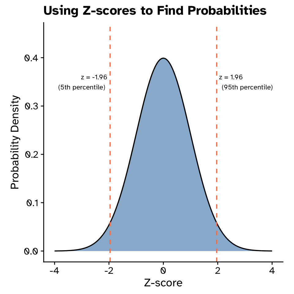
Probability distributions
Normal distribution: Z-scores
Probability distributions
Normal distribution as a model
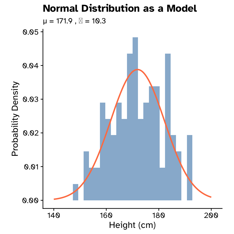
Probability distributions
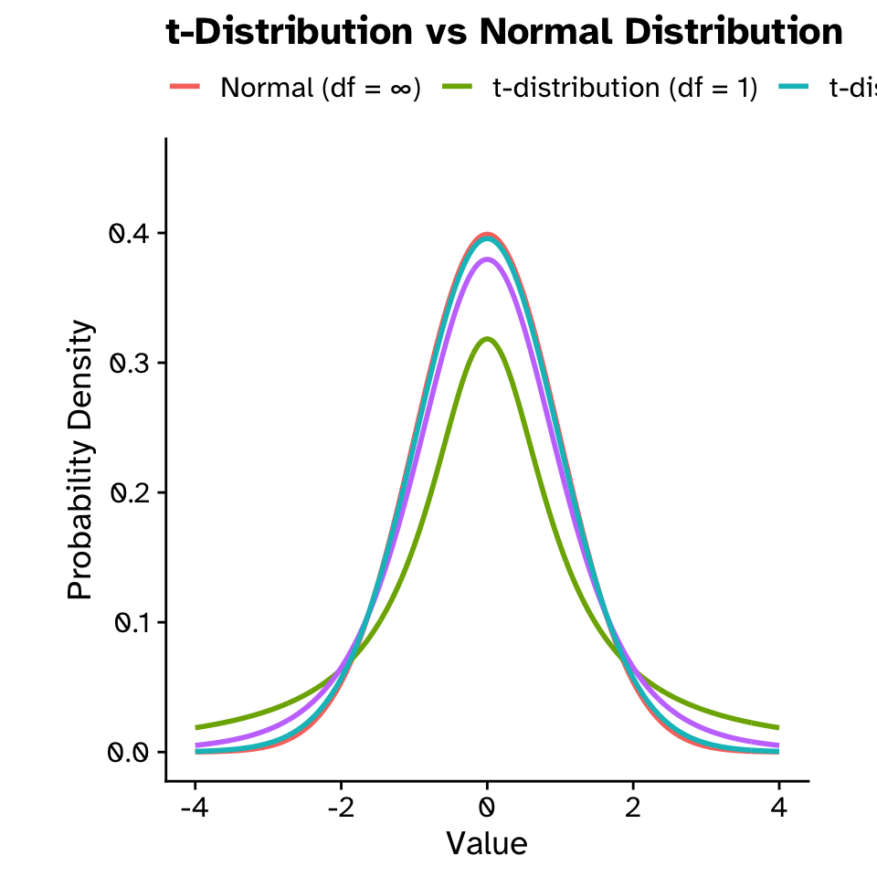
Normal distribution as a model (t-distribution)
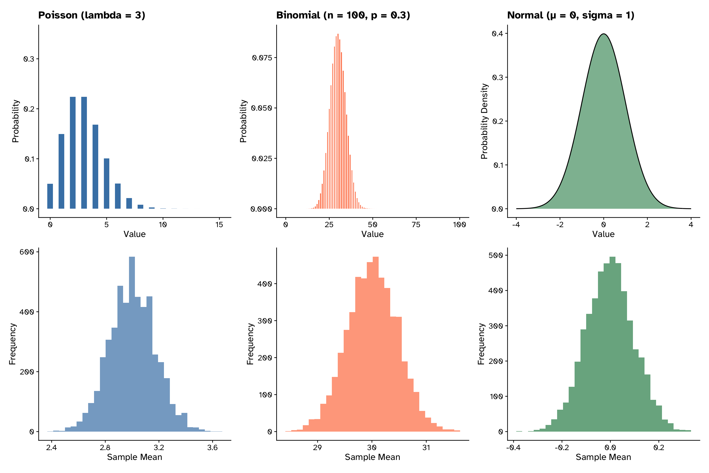
Central limit theorem
The distribution of means is normal
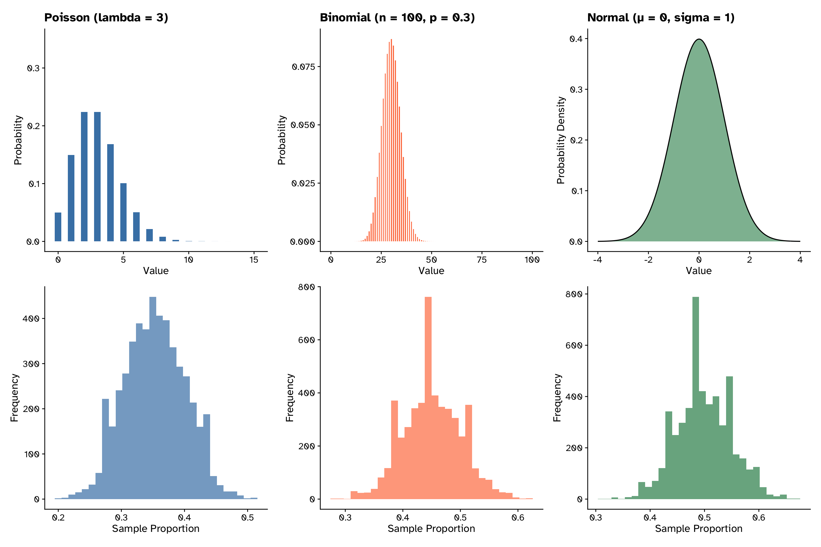
Central limit theorem
The distribution of proportions is normal
Central limit theorem
The distribution of slopes is normal
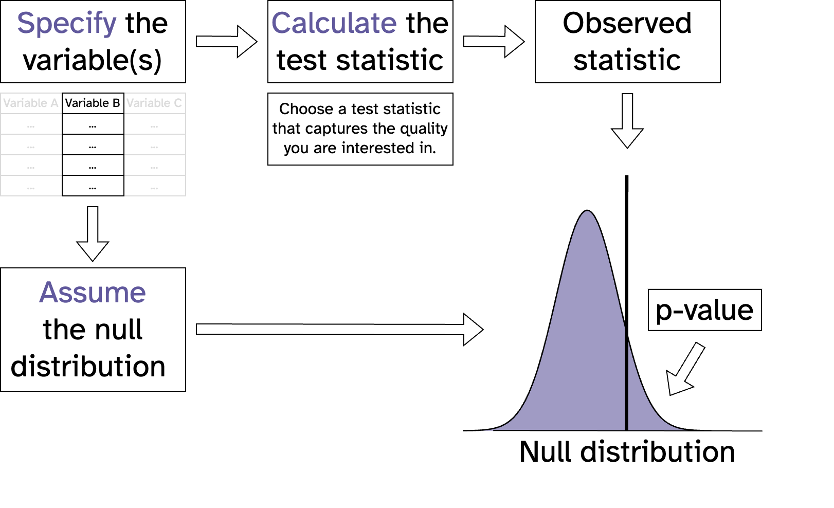
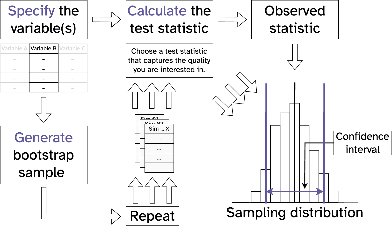
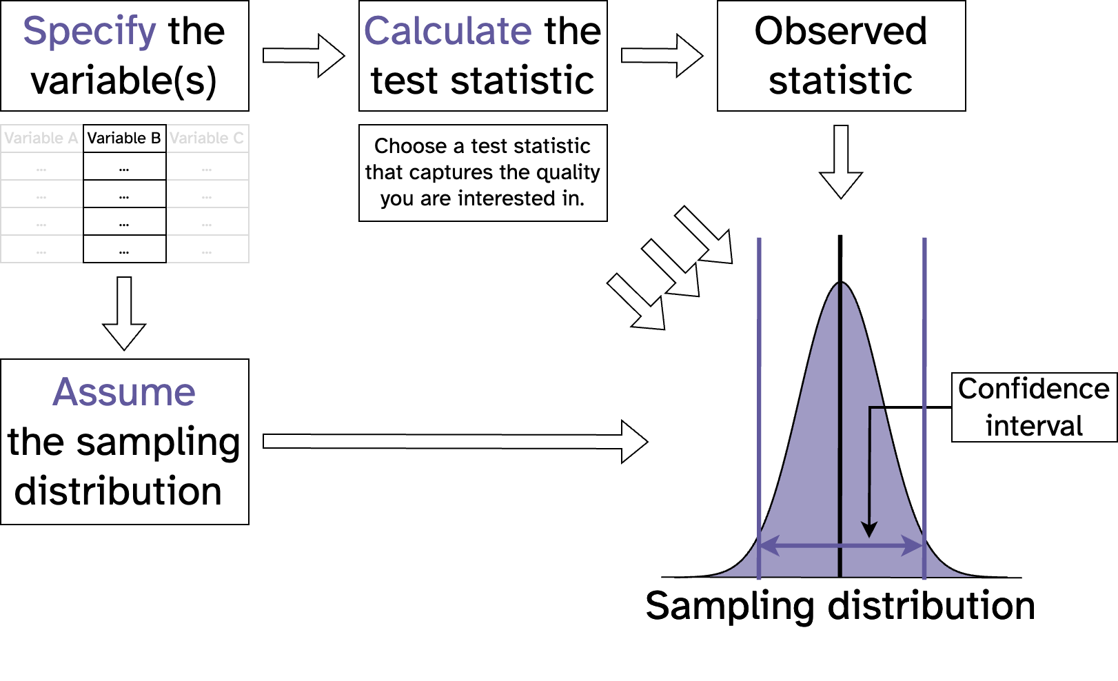
Statistical inference with maths
Resampling vs maths
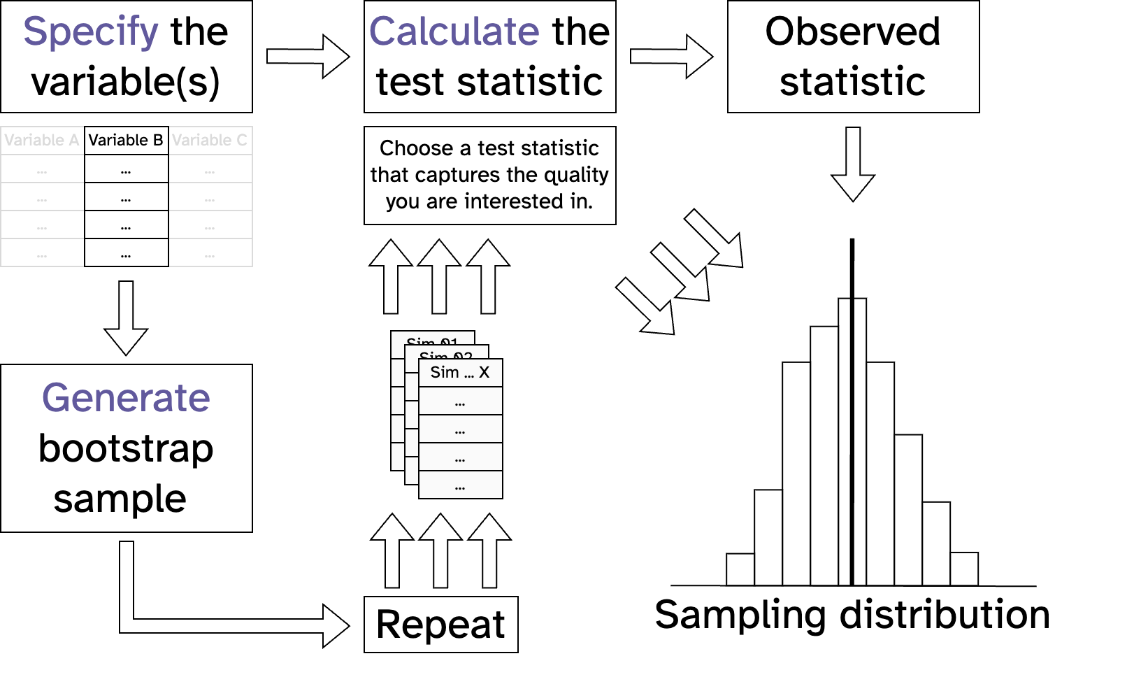
Statistical inference with maths
Resampling vs maths
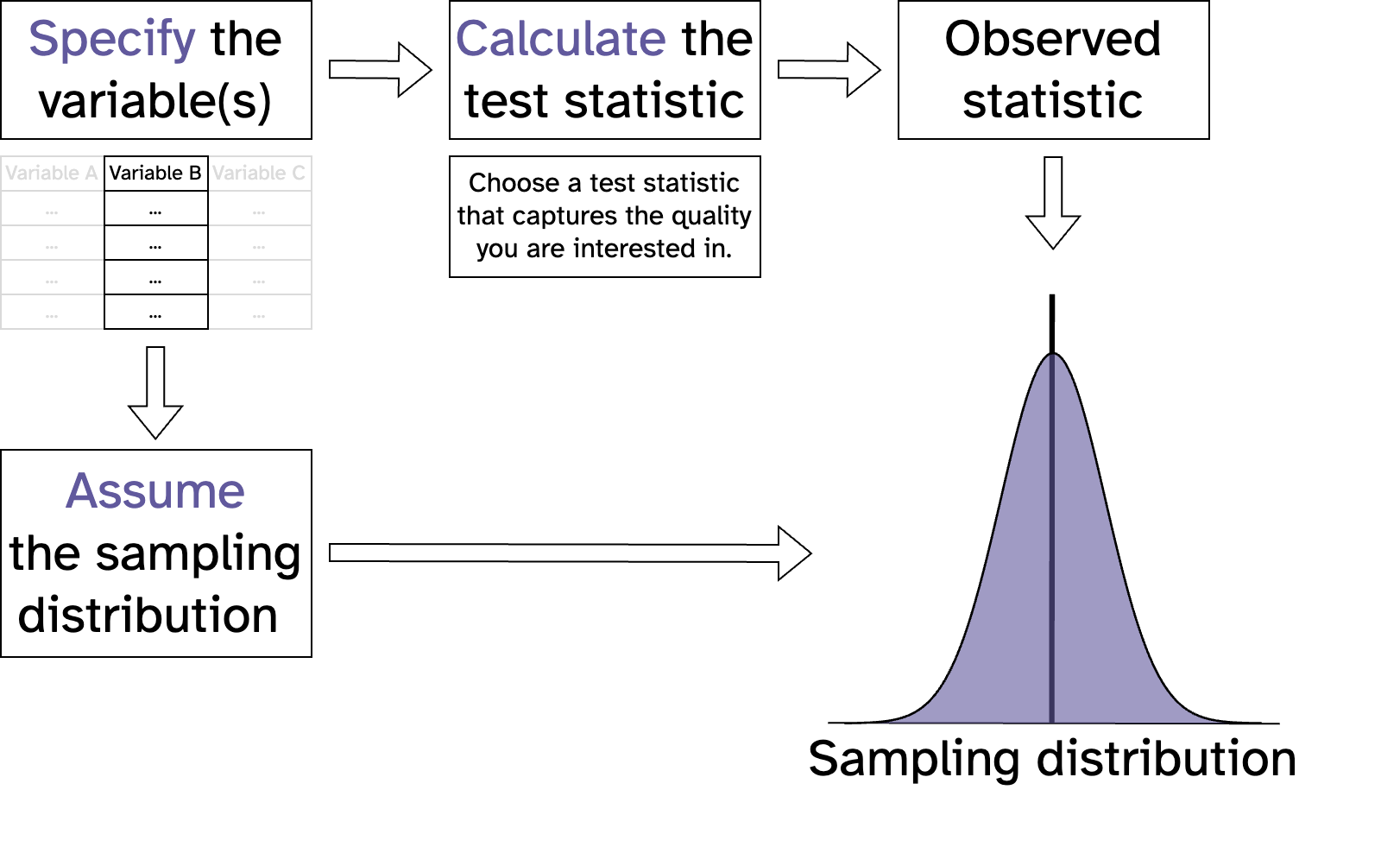
Statistical inference with maths
Resampling vs maths

Statistical inference with maths
Resampling vs maths (diff in means CI)
- What is the difference in average size of males and females?
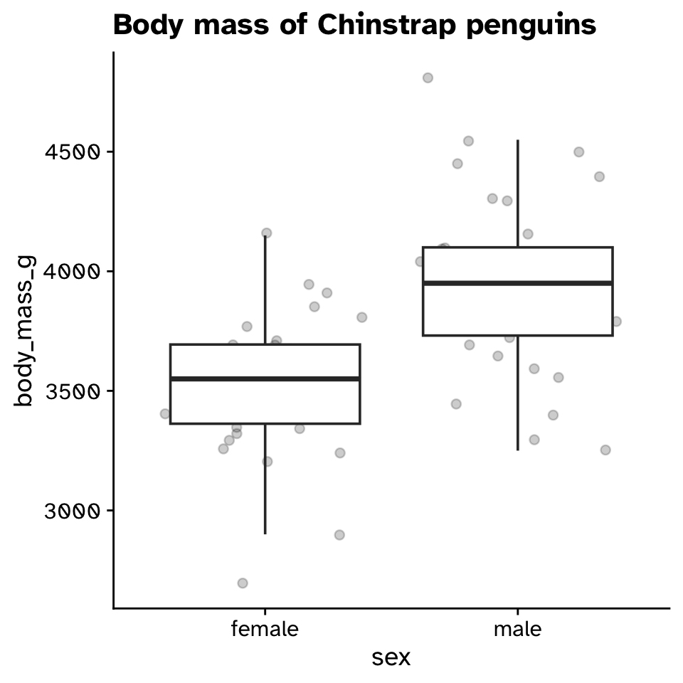
Statistical inference with maths
Resampling vs maths (diff in means CI)
Statistical inference with maths
Resampling vs maths (diff in means CI)
Statistical inference with maths
Resampling vs maths (diff in means CI)
Statistical inference with maths
Resampling vs maths (diff in means CI)
Statistical inference with maths
Resampling vs maths (\(\chi^2\) Goodness of fit)
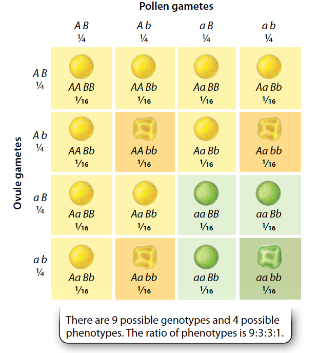
Statistical inference with maths
Resampling vs maths (\(\chi^2\) Goodness of fit)
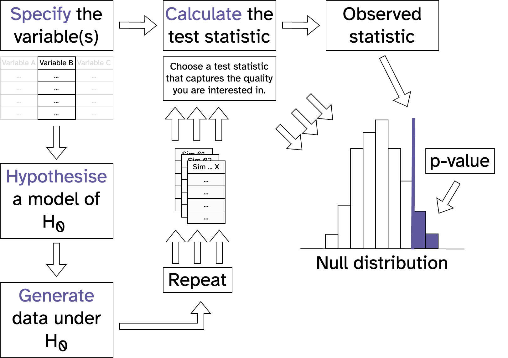
Statistical inference with maths
Resampling vs maths (\(\chi^2\) Goodness of fit)