Correlation, Causation, and Linear Regression
Lecture 8
2025-04-04
Correlation
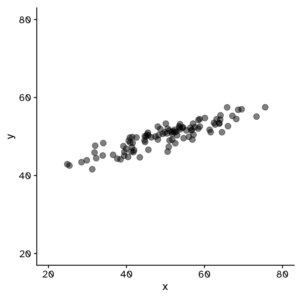
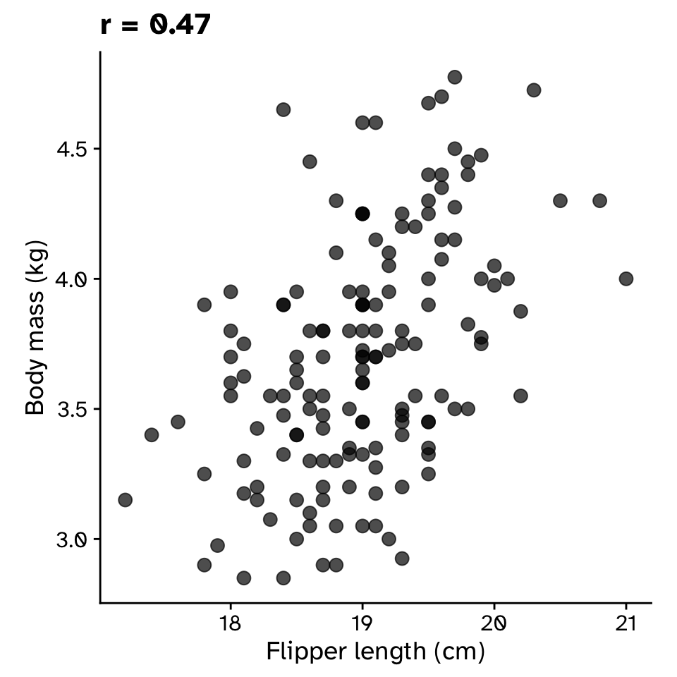
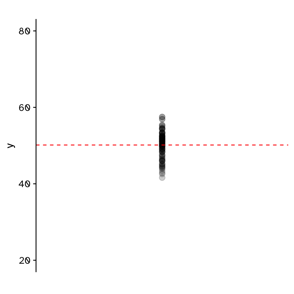
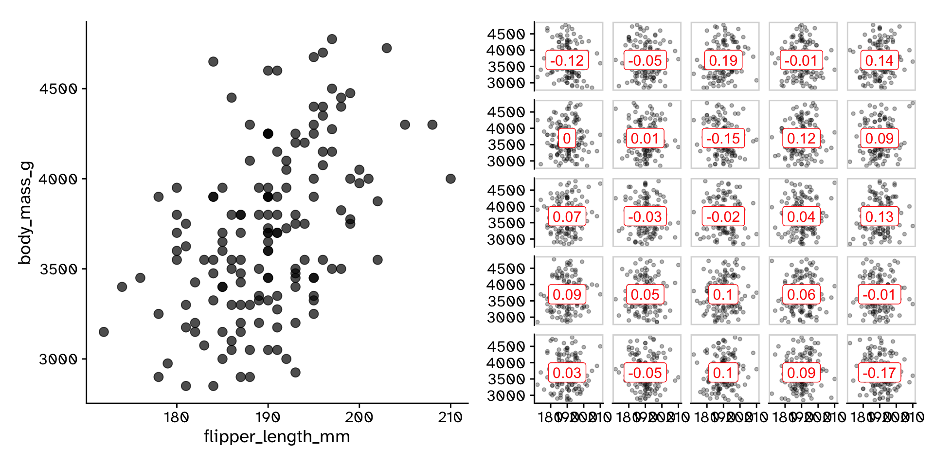
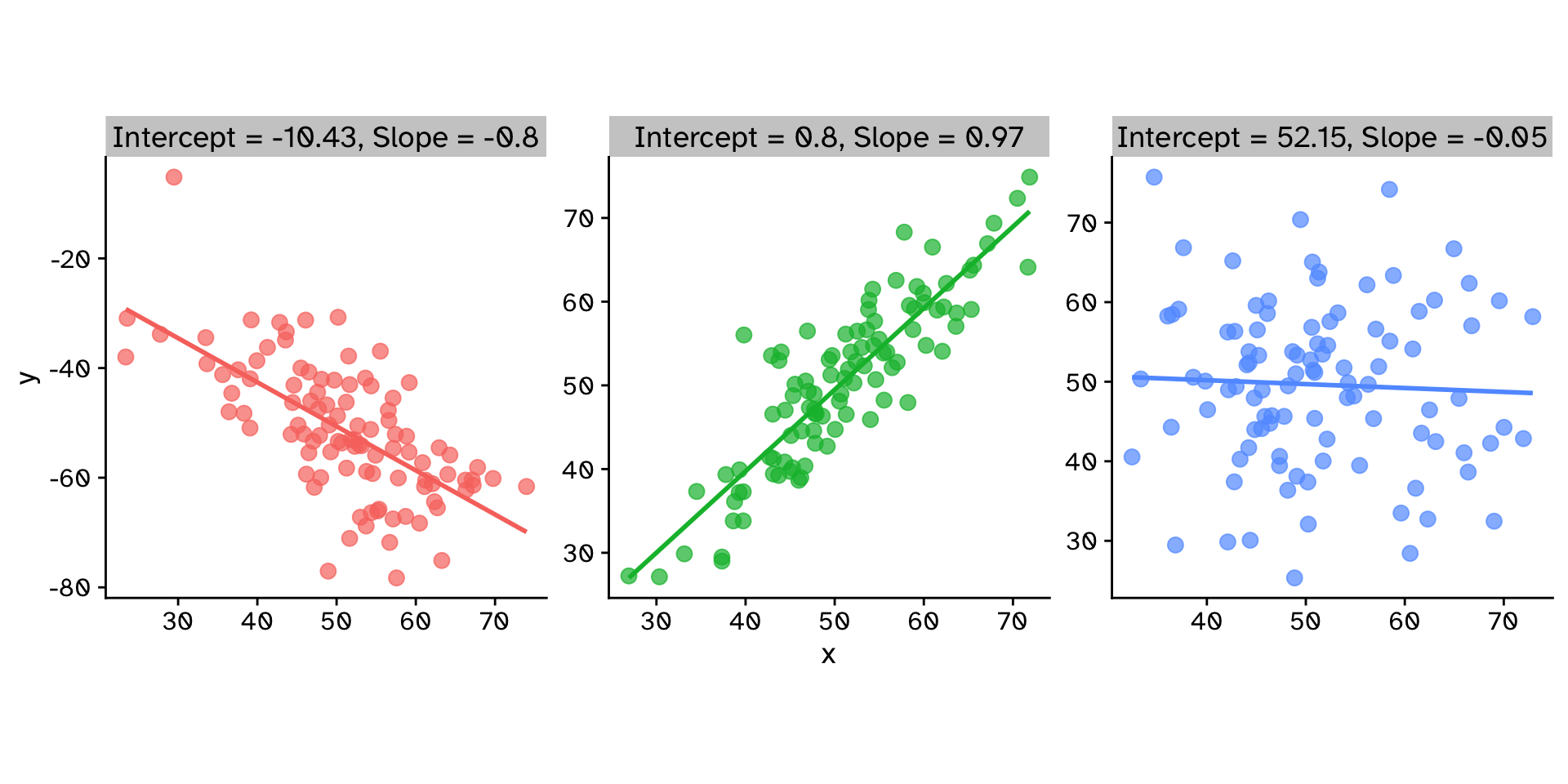
Do two continuous variables covary?
Correlation
Do two continuous variables covary?
Correlation
Do two continuous variables covary?
Correlation
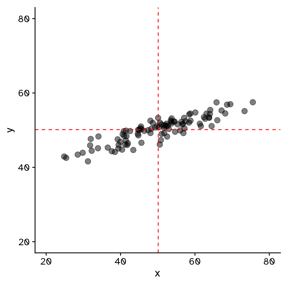
Do two continuous variables covary?
Correlation
Do two continuous variables covary?

Correlation
Do two continuous variables covary?

Correlation
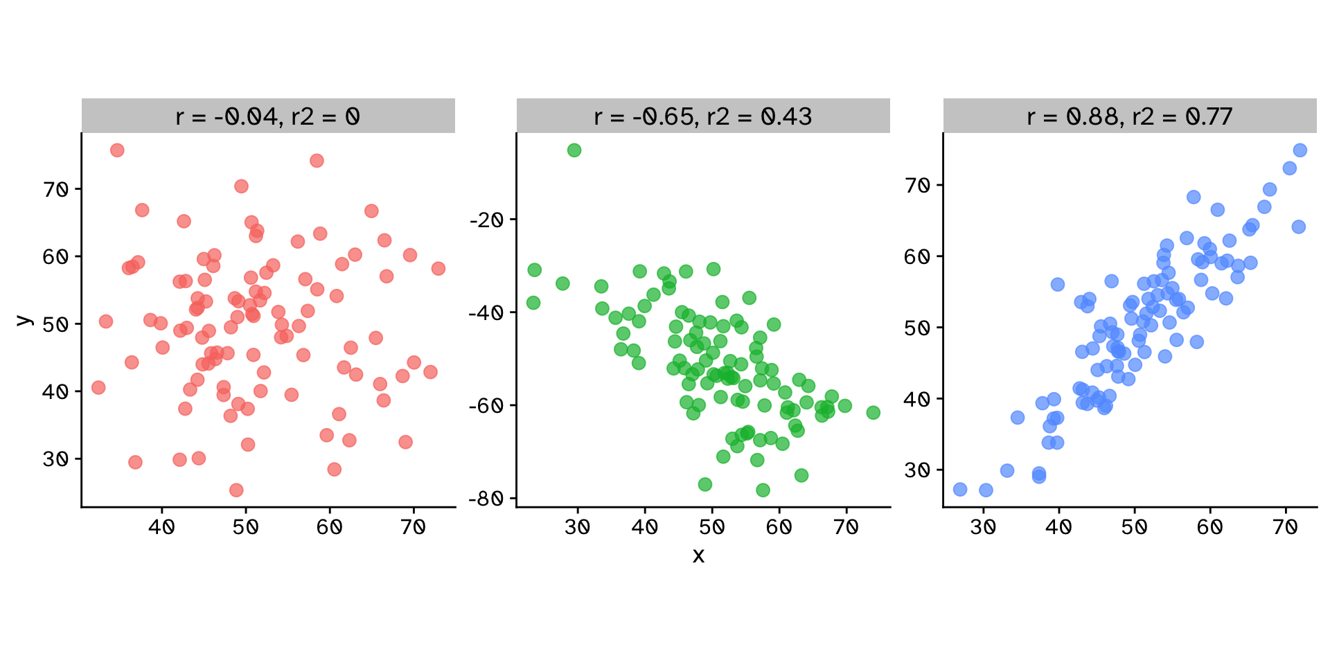
Do two continuous variables covary?
Correlation
Do two continuous variables covary?
Correlation
Confidence intervals
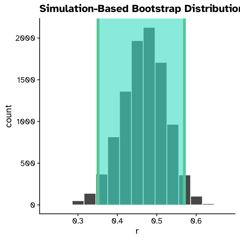
Correlation
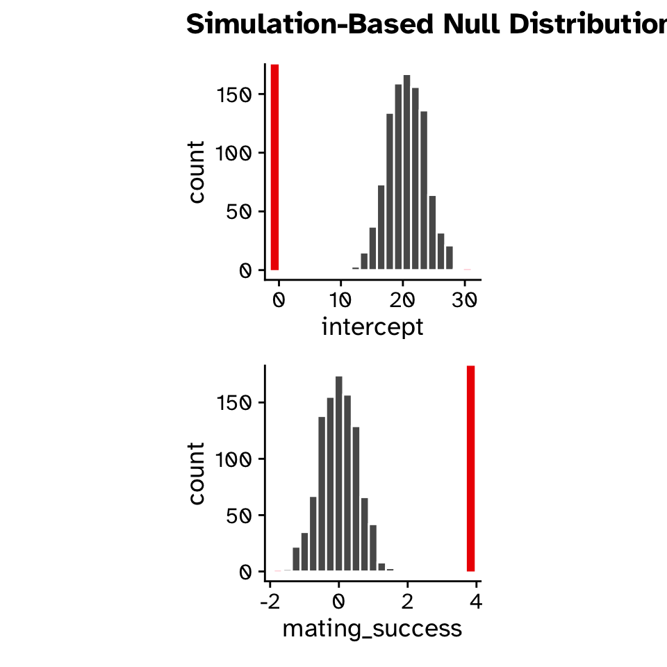
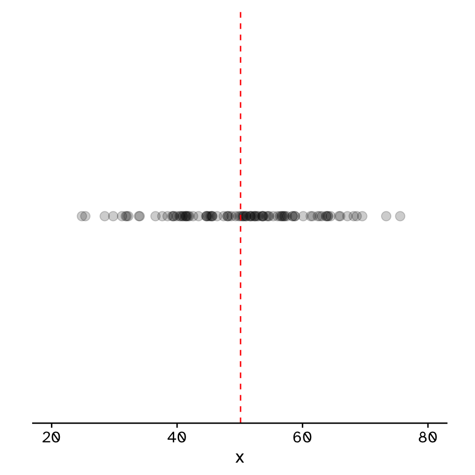
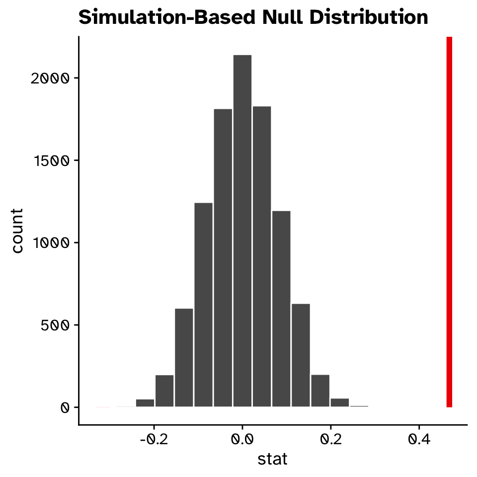
Hypothesis test
- How could we generate a null distribution?

Correlation
Hypothesis test
Correlation
Hypothesis test
Regression
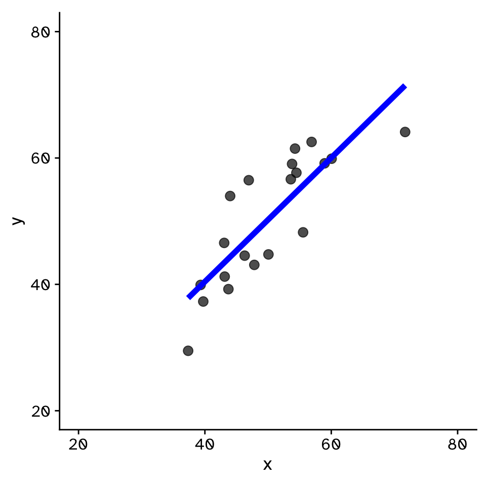
How does variable Y depend on variable X
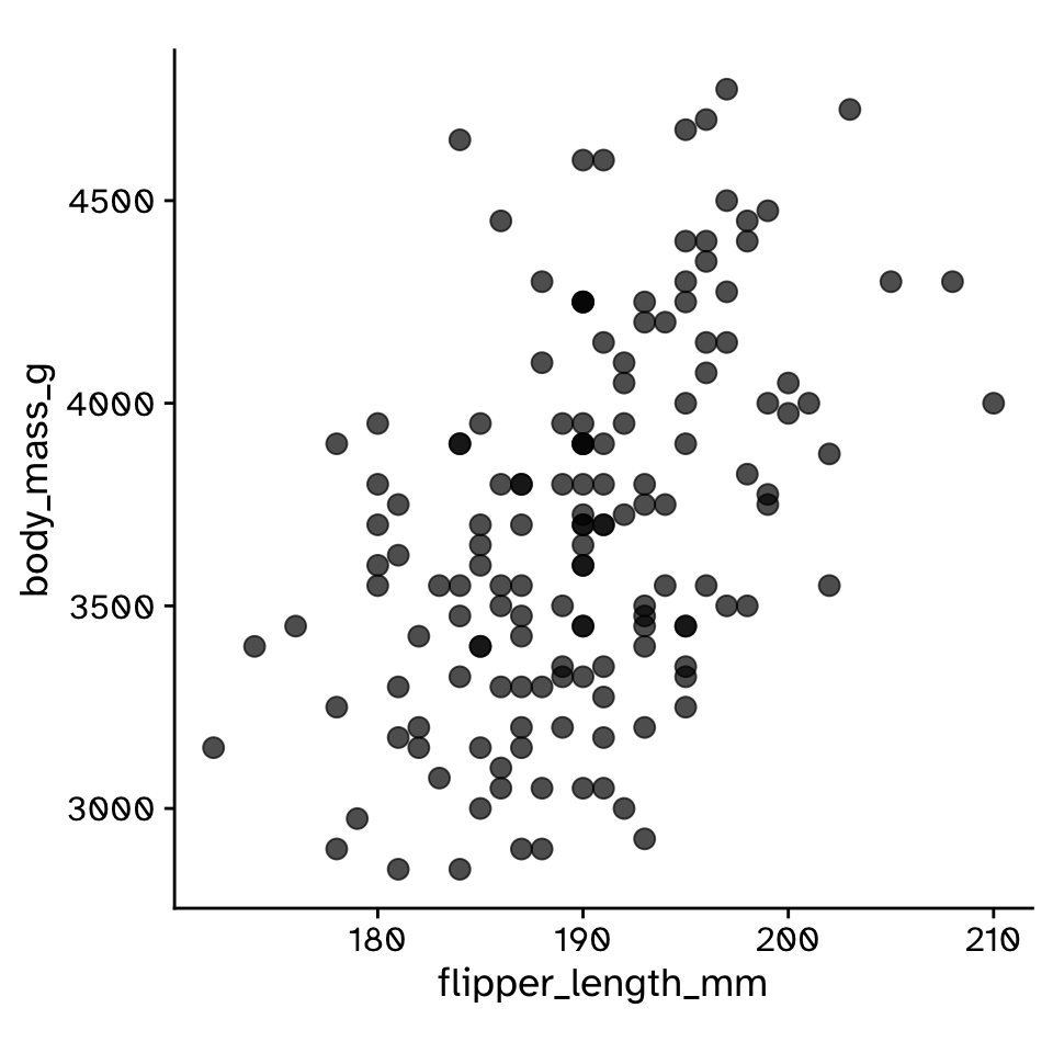
Regression
How does variable Y depend on variable X
Regression
How does variable Y depend on variable X
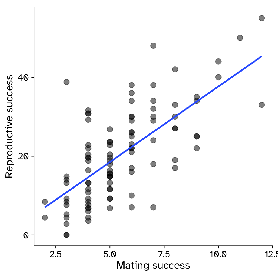
- Example: For sexual selection to operate, an increase in mating success (number of mates) must result in an increase in reproductive success (number of offspring).
Regression
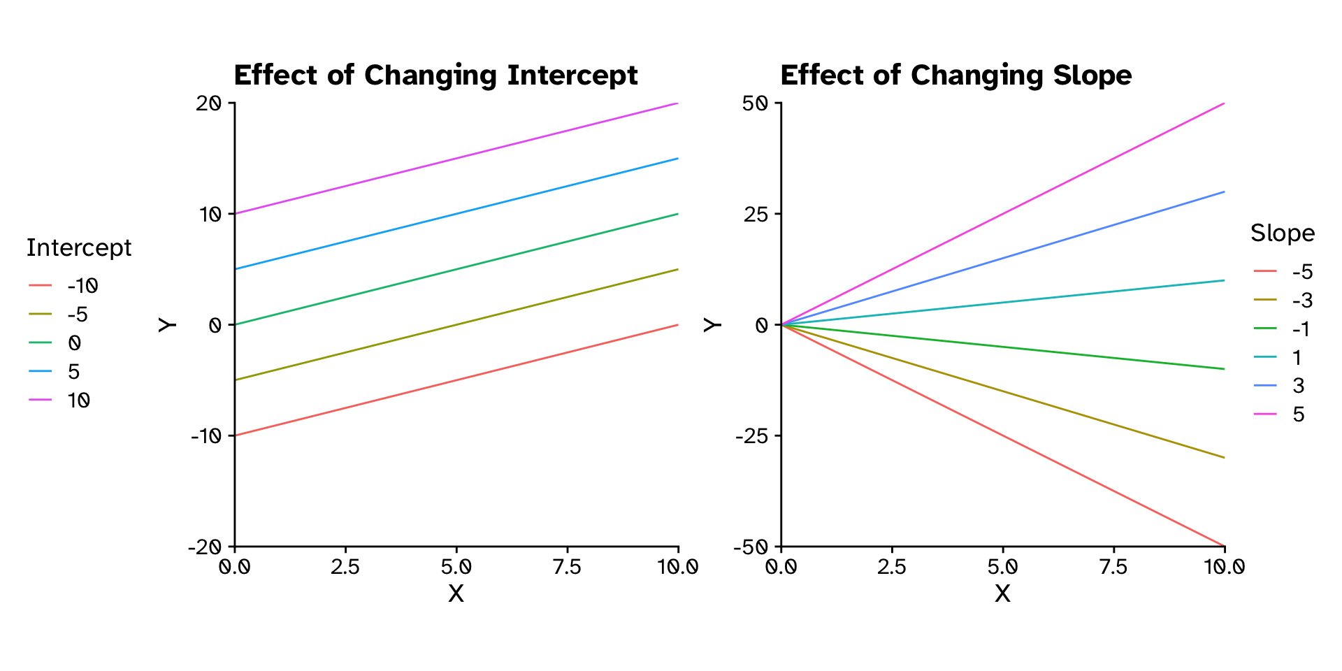
How does variable Y depend on variable X
\[ y = \beta_1x+\beta_0 \]
\[ y = 3.83x-0.68 \]
- \(\beta_1\) = strength of sexual selection
- For each additional mate, an individual (on average) gains \(\beta_1\) additional offspring
- For 5 mates (\(x=5\)):
- \(y = 3.83\times5-0.68\)
- \(y = 18.47\)

Regression
How does variable Y depend on variable X
Regression
How does variable Y depend on variable X
Regression
How does variable Y depend on variable X
Regression
How does variable Y depend on variable X
Regression
How does variable Y depend on variable X

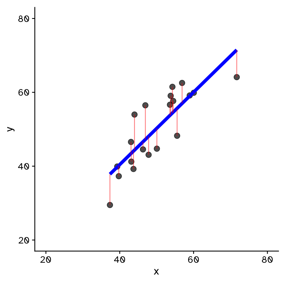
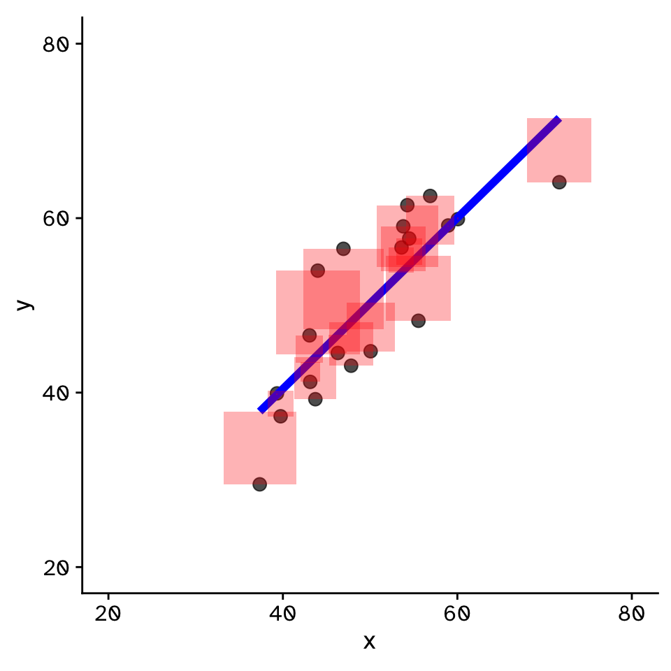
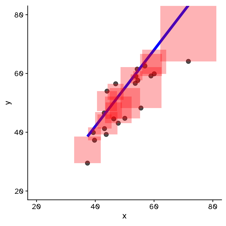
- Fit by solving to minimise the sum of the squared residuals (SSR)
- Find \(\beta_1\) and \(\beta_0\) that minimise the SSR
- Called a “loss function”
- Many approaches to do this!
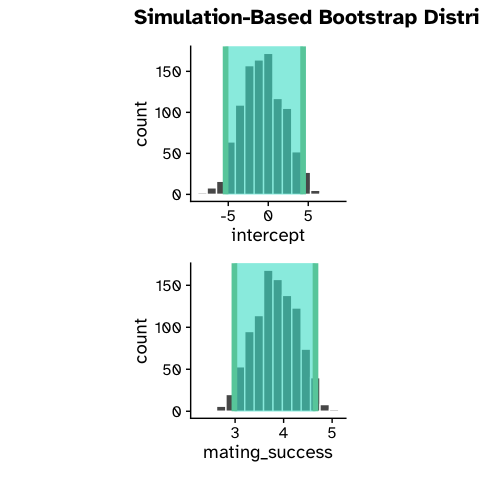
Regression
Confidence intervals
Regression
Hypothesis test