Computational statistics
Lecture 2
2026-04-28
Review
Populations and Samples

Review
Populations and Samples
Review
Populations and Samples
Review
Populations and Samples
Review
Populations and Samples
Review
The sampling distribution

Review
The sampling distribution
- Problem: we (usually) only collect one sample
Review
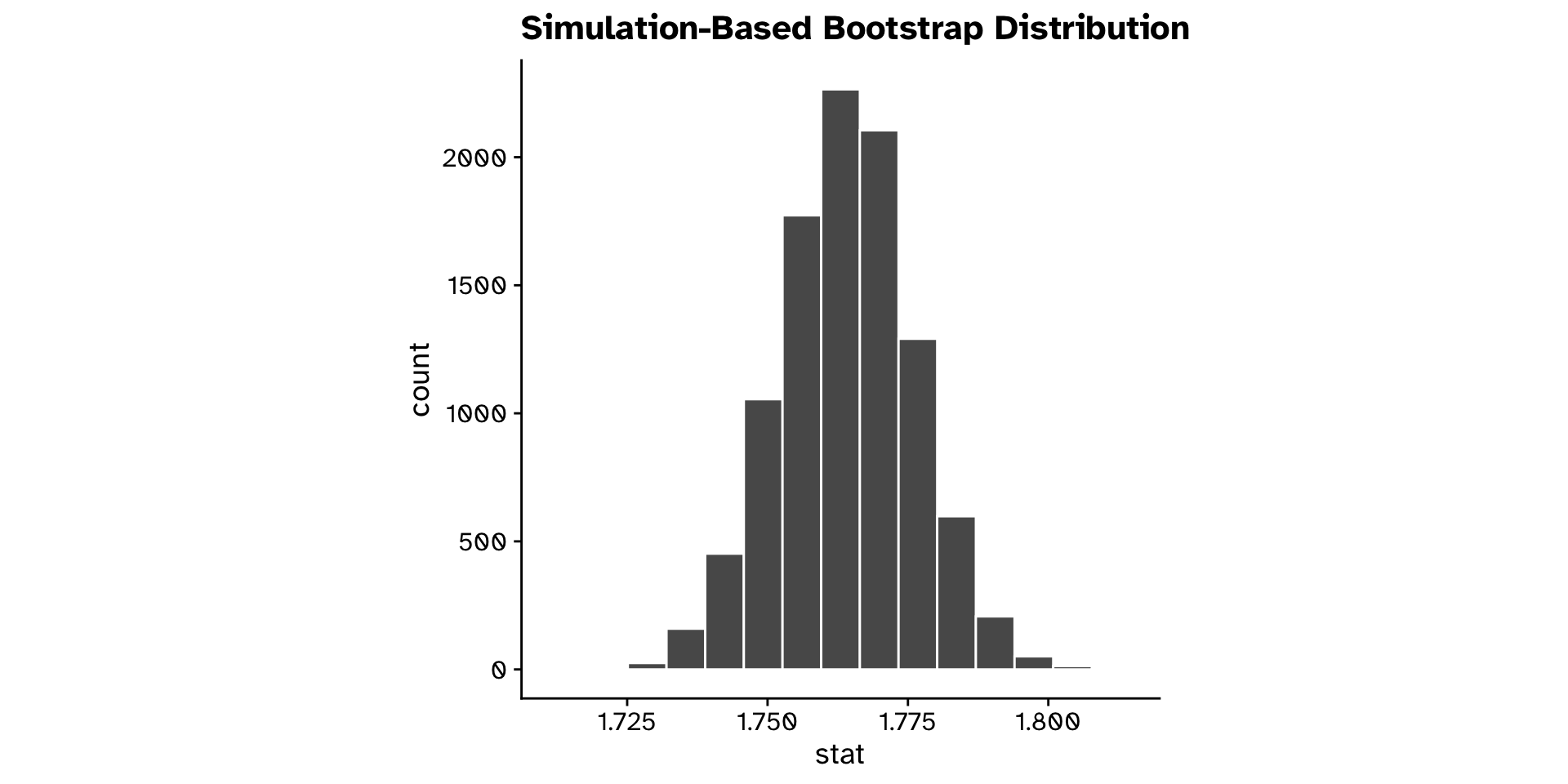
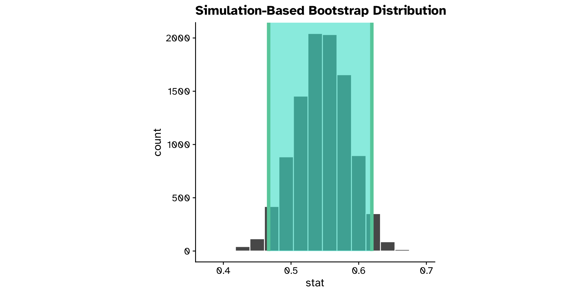
The bootstrap sampling distibution

Review
The bootstrap sampling distibution
Review
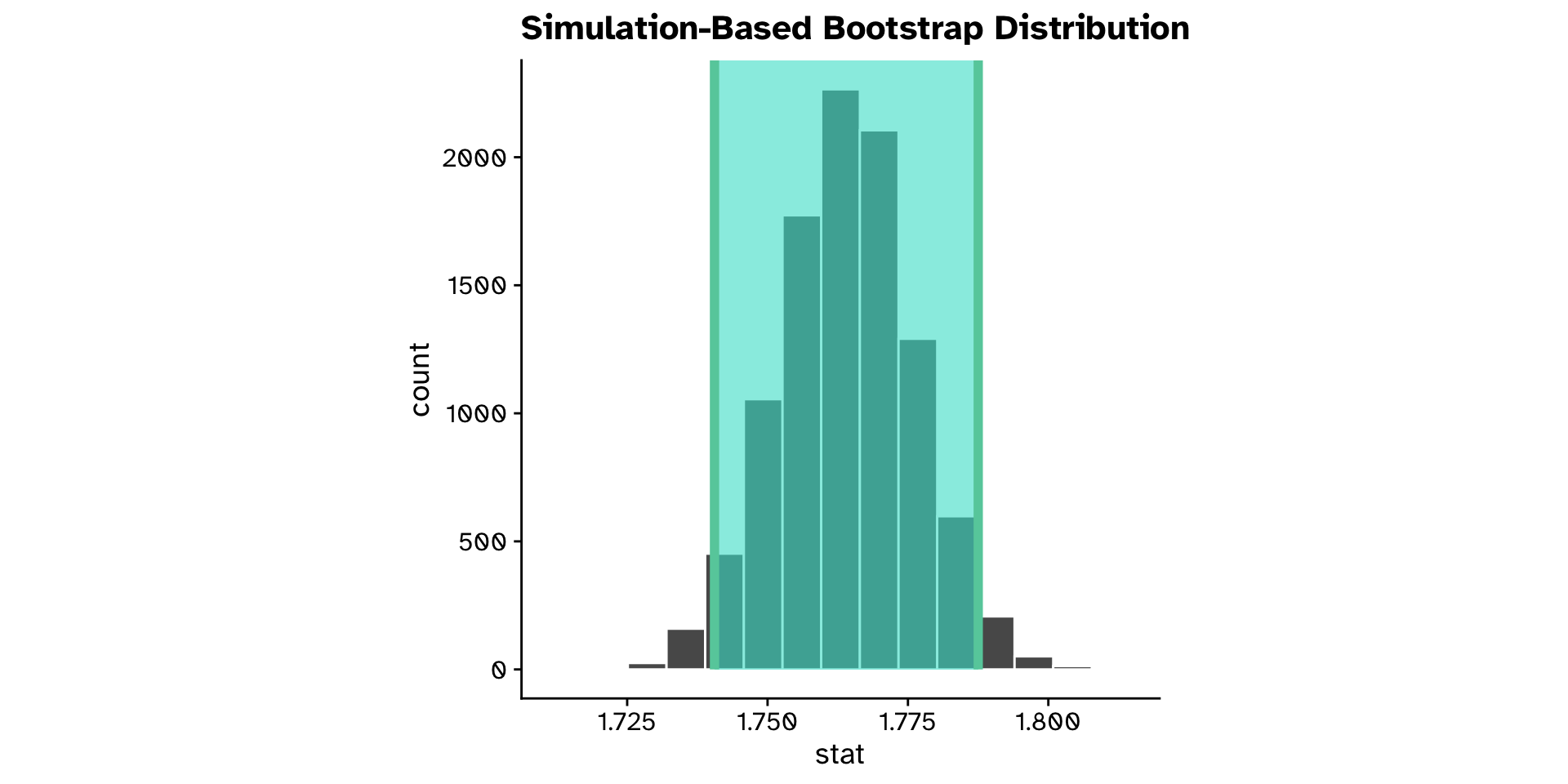
Confidence intervals

Review
Confidence intervals
Review
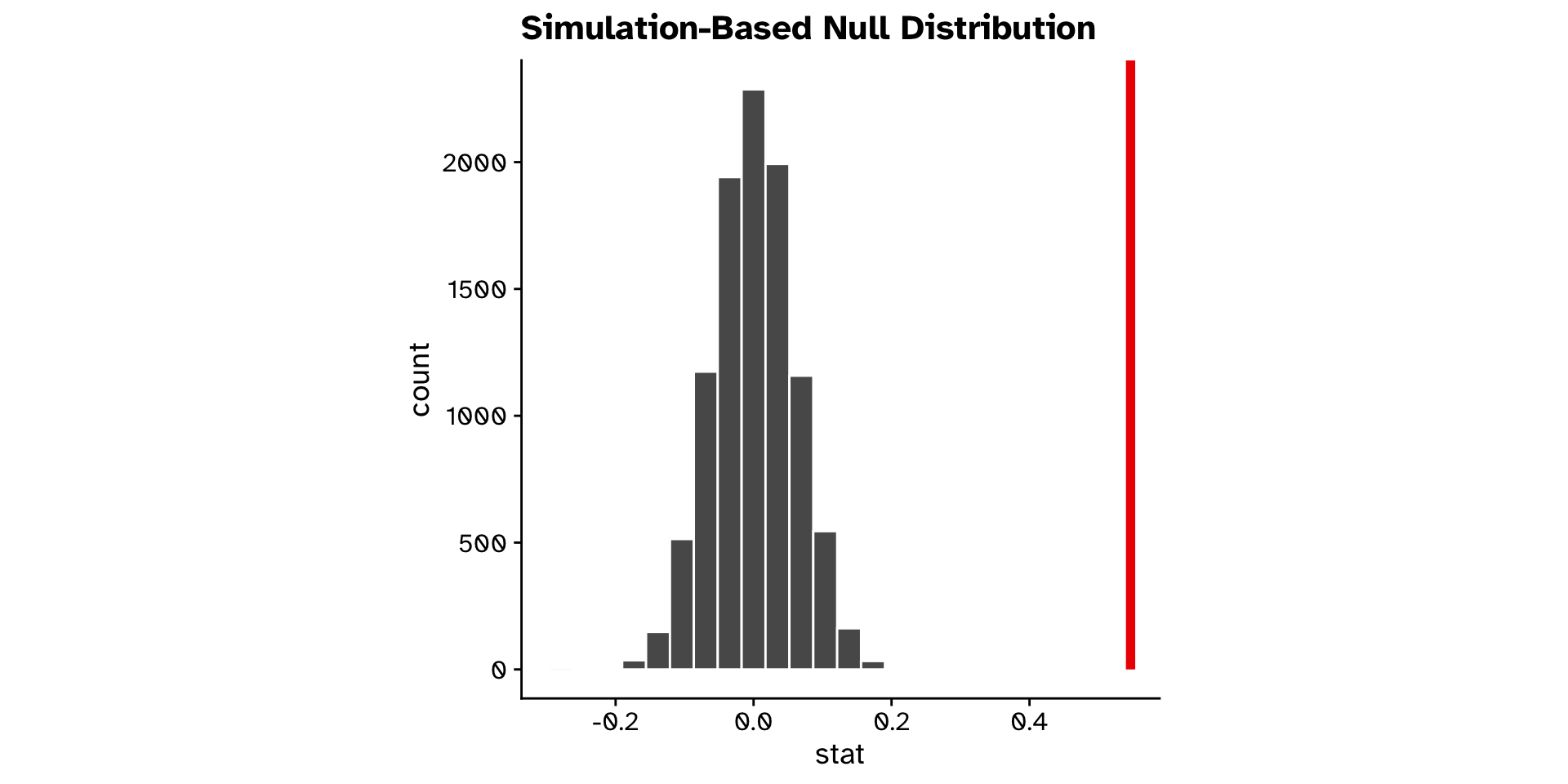
Hypothesis testing

Review
Hypothesis testing
Review
Hypothesis testing

Review
Hypothesis testing
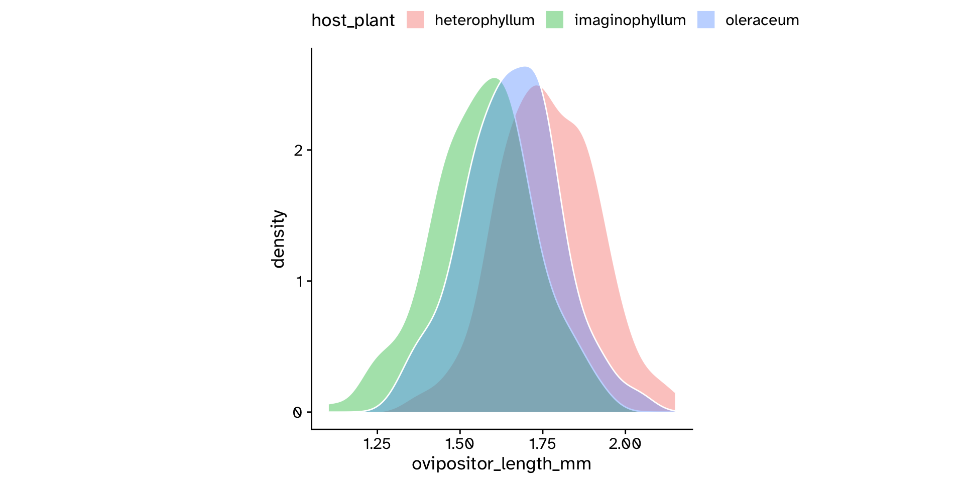
Comparing means between >2 groups
Analysis of Variance (ANOVA)
Comparing means between >2 groups
Analysis of Variance (ANOVA)
Comparing means between >2 groups
Analysis of Variance (ANOVA)
Comparing means between >2 groups
Analysis of Variance (ANOVA)
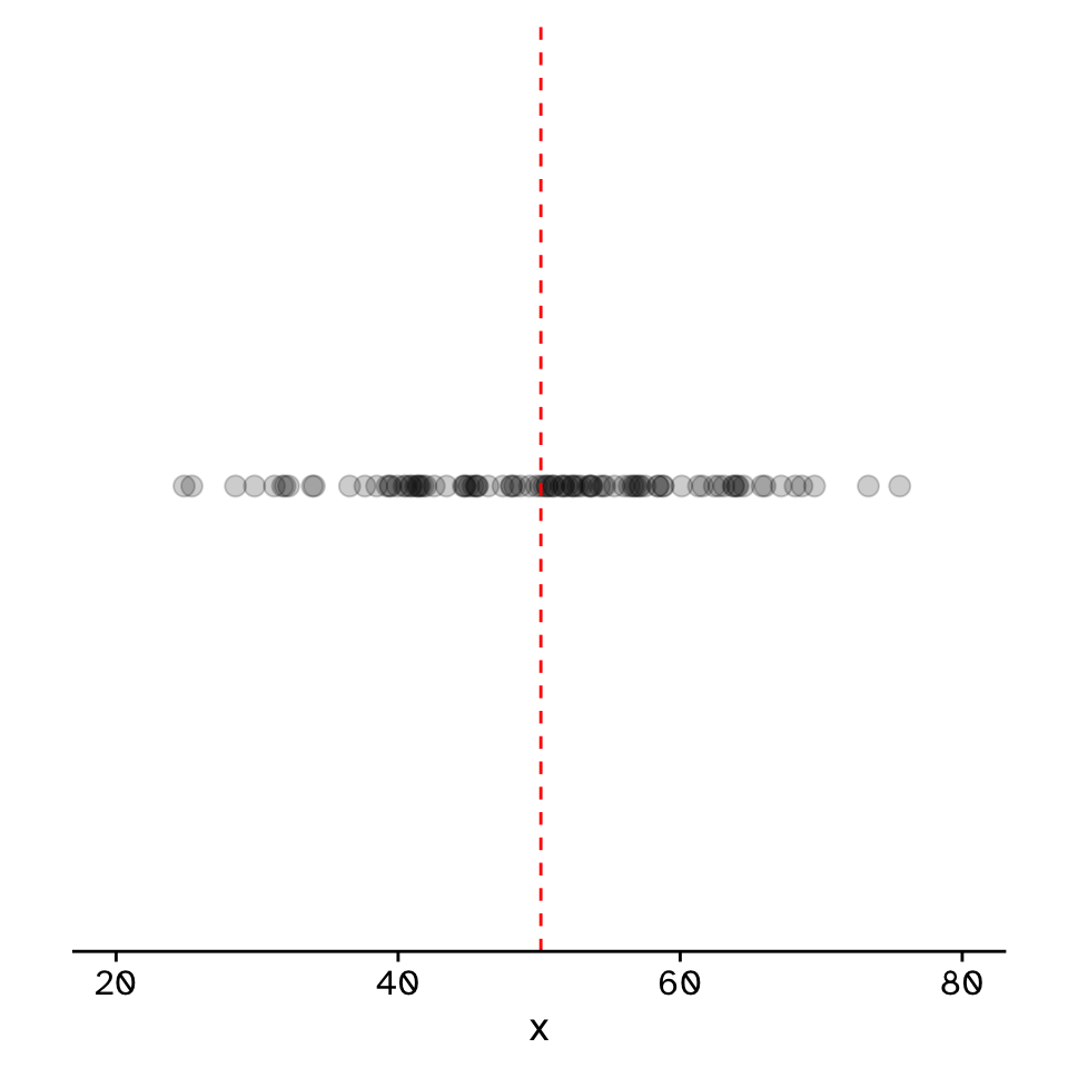
Different from a hypothesised value?
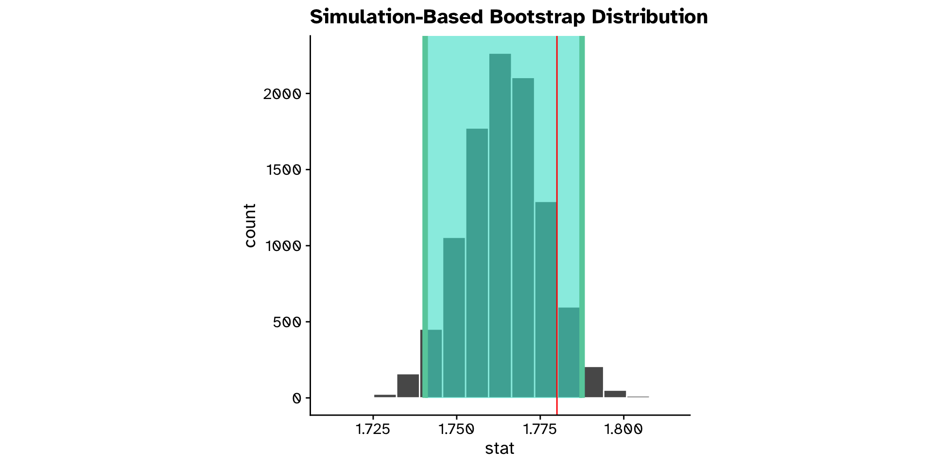
Continuous variable (confidence interval approach)
Different from a hypothesised value?
Continuous variable (confidence interval approach)
Different from a hypothesised value?
Continuous variable (confidence interval approach)
Different from a hypothesised value?
Continuous variable (confidence interval approach)
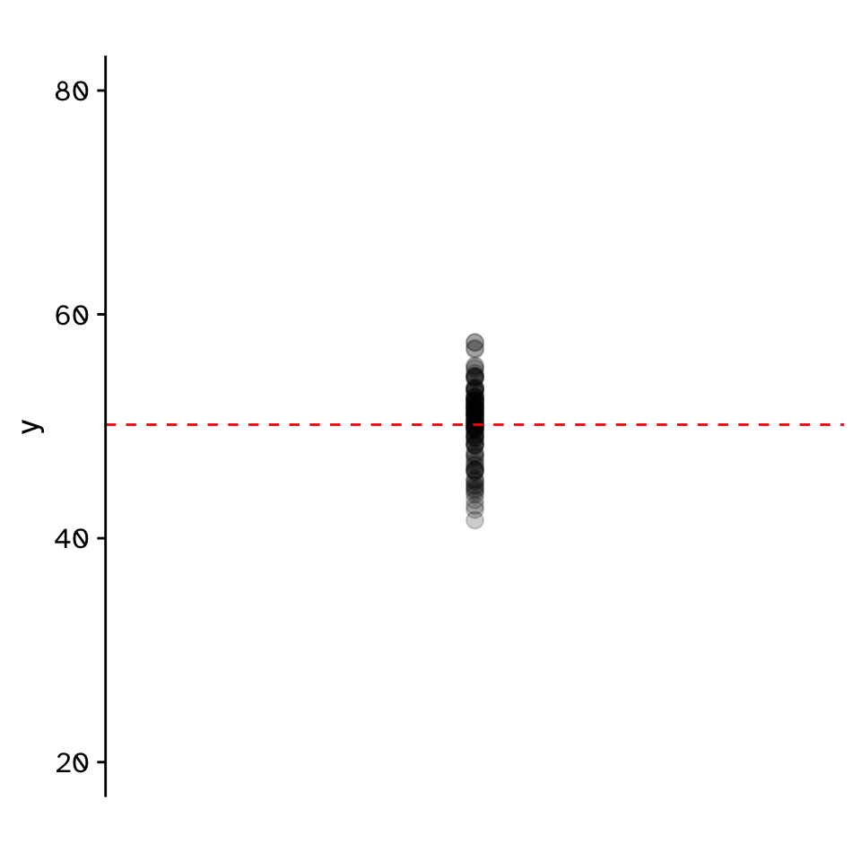
Different from a hypothesised value?
Continuous variable (hypothesis testing approach)
Different from a hypothesised value?
Continuous variable (hypothesis testing approach)
Different from a hypothesised value?
Continuous variable (hypothesis testing approach)
Different from a hypothesised value?
Continuous variable (hypothesis testing approach)
Different from a hypothesised value?
Continuous variable (hypothesis testing approach)
Different from a hypothesised value?
Continuous variable (hypothesis testing approach)
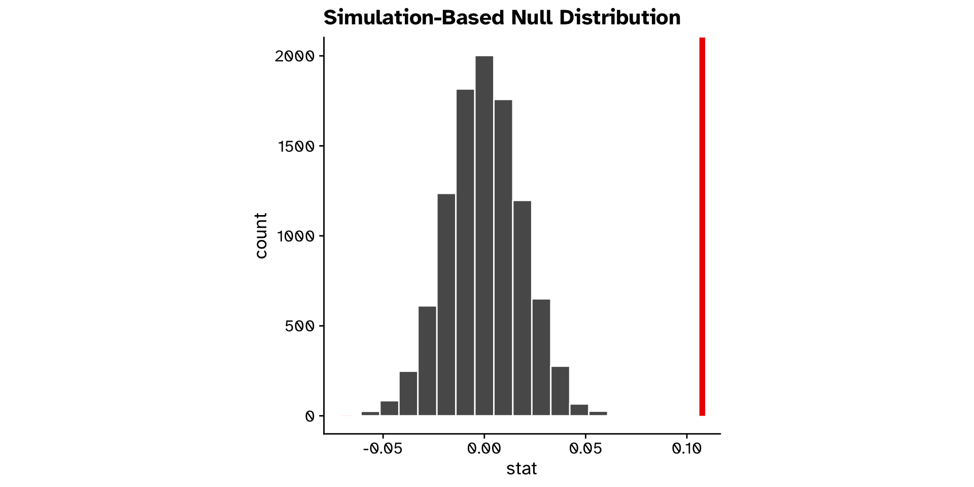
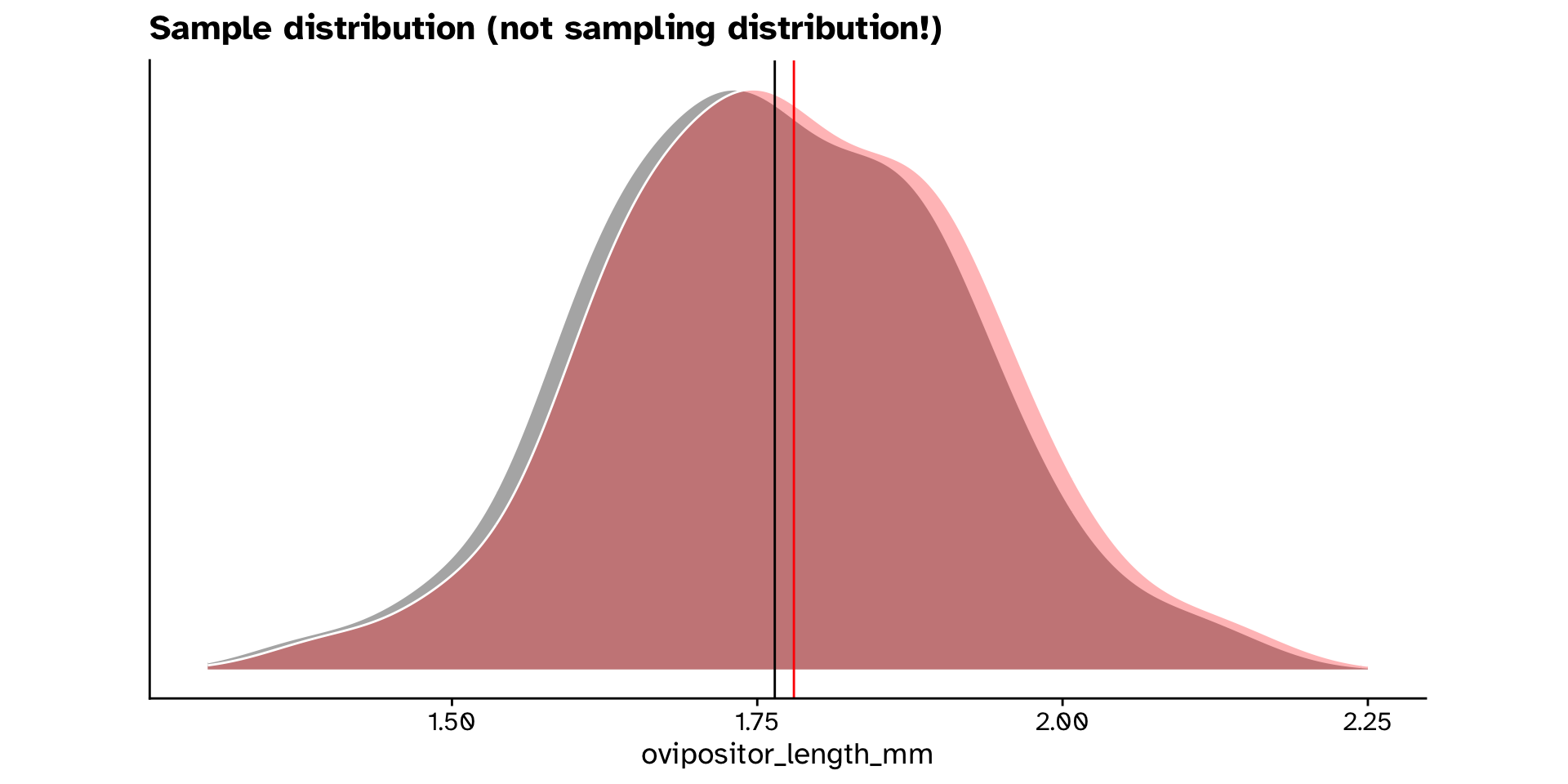
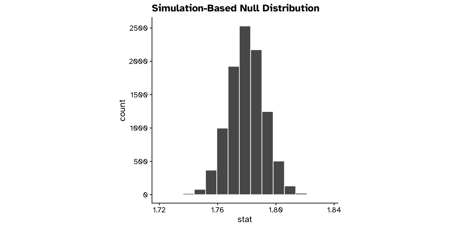
- Bootstrap resample from our new dataset that is compatible with the null hypothesis
Different from a hypothesised value?
Continuous variable (hypothesis testing approach)
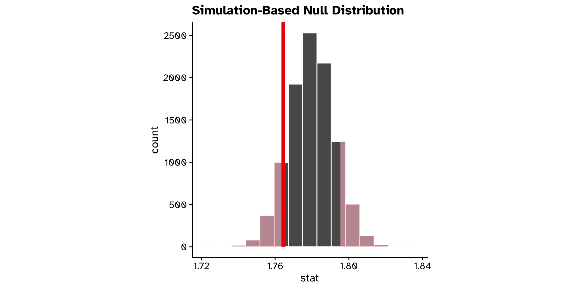
- Compare with observed value

Different from a hypothesised value?
Continuous variable (hypothesis testing approach)
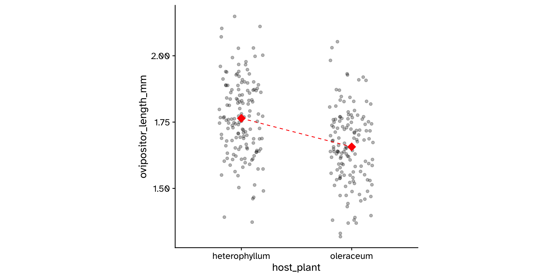
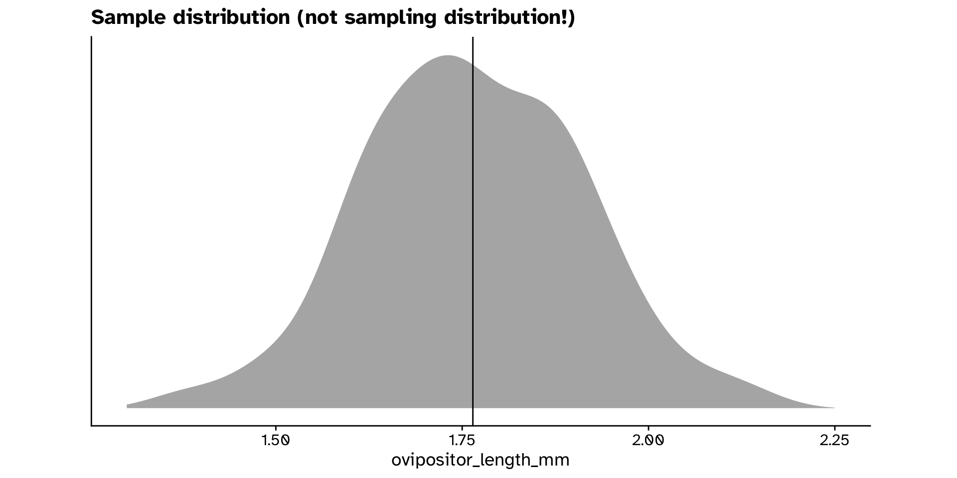
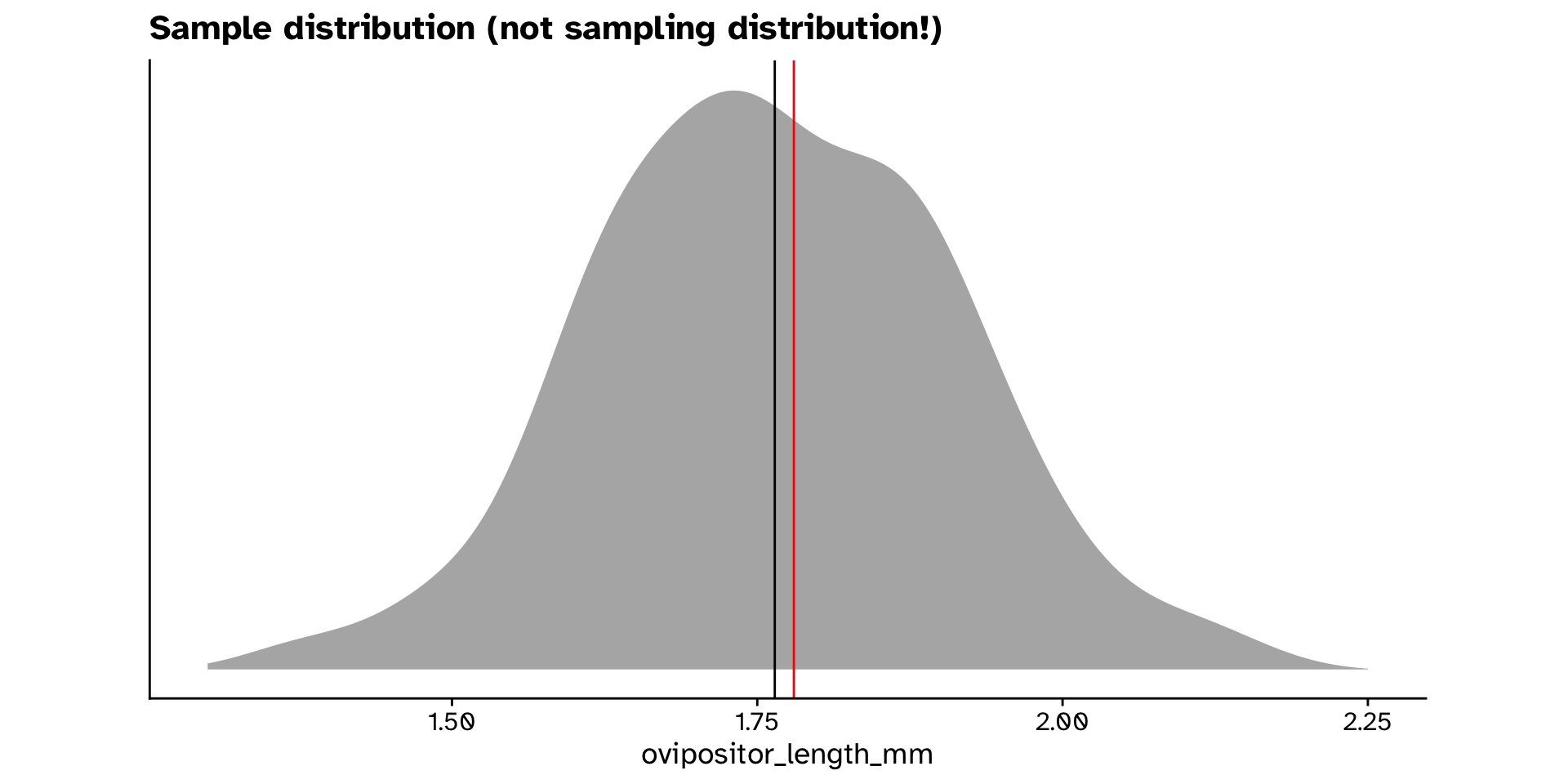
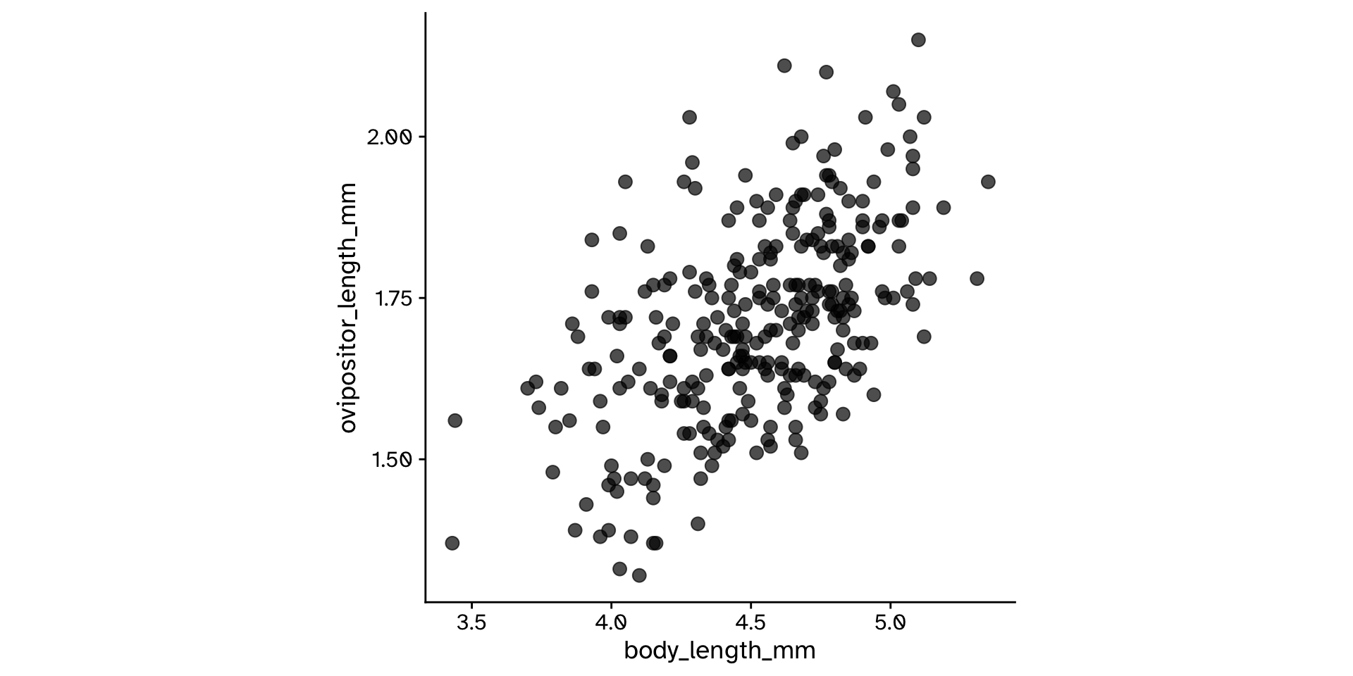
- Is the mean
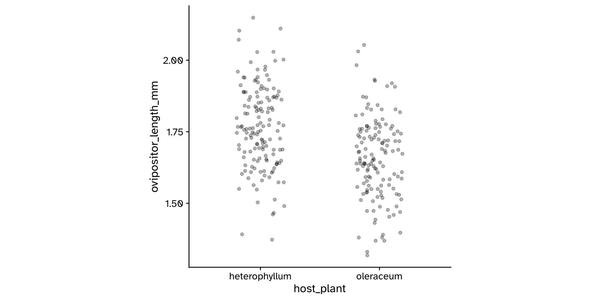
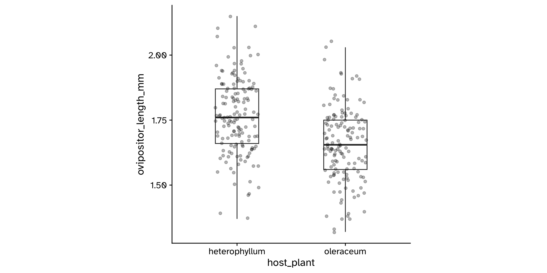
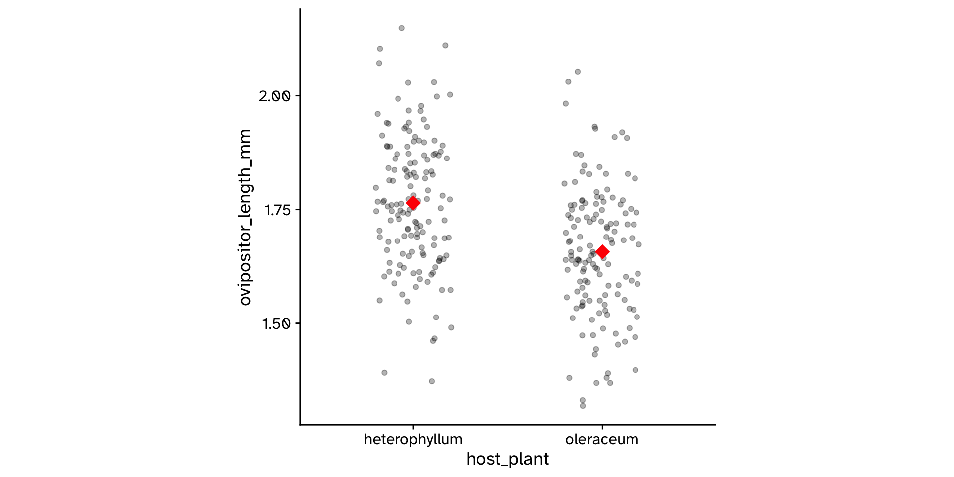
ovipositor_length_mmin theheterophyllumhost race different from 1.78 mm?- Observed: 1.764 mm
- If the true mean was 1.78 mm, probability to observe 1.764 mm or a value more extreme is 0.2 (20% chance)
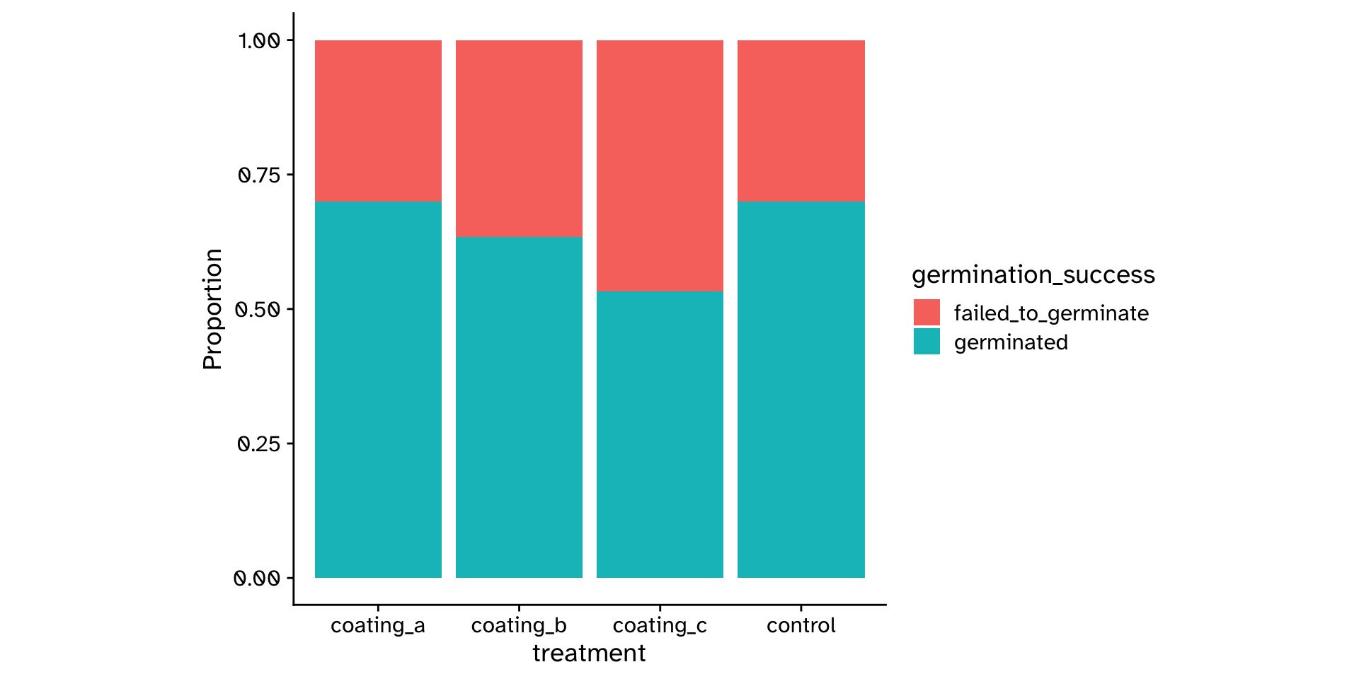
Tests of proportion
Is a proportion different from a hypothesised value?
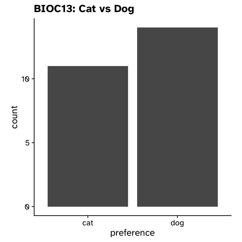
Tests of proportion
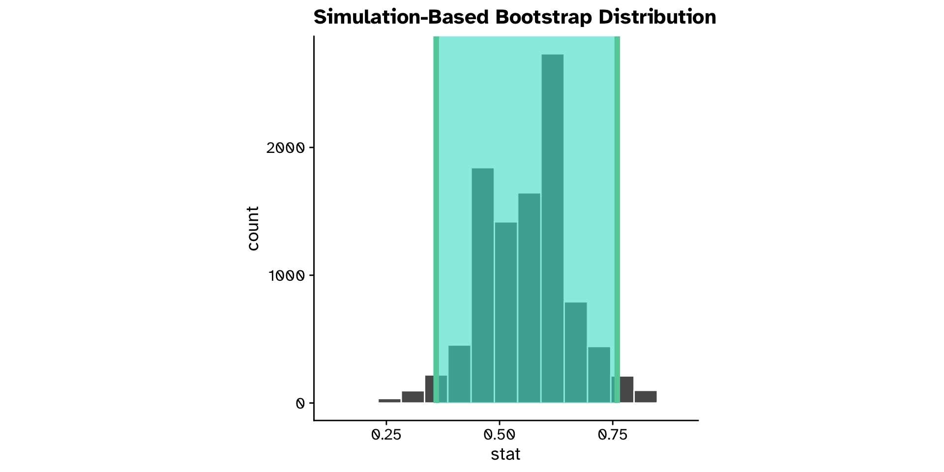
Is a proportion different from a hypothesised value? (CI)
Tests of proportion
Is a proportion different from a hypothesised value? (CI)
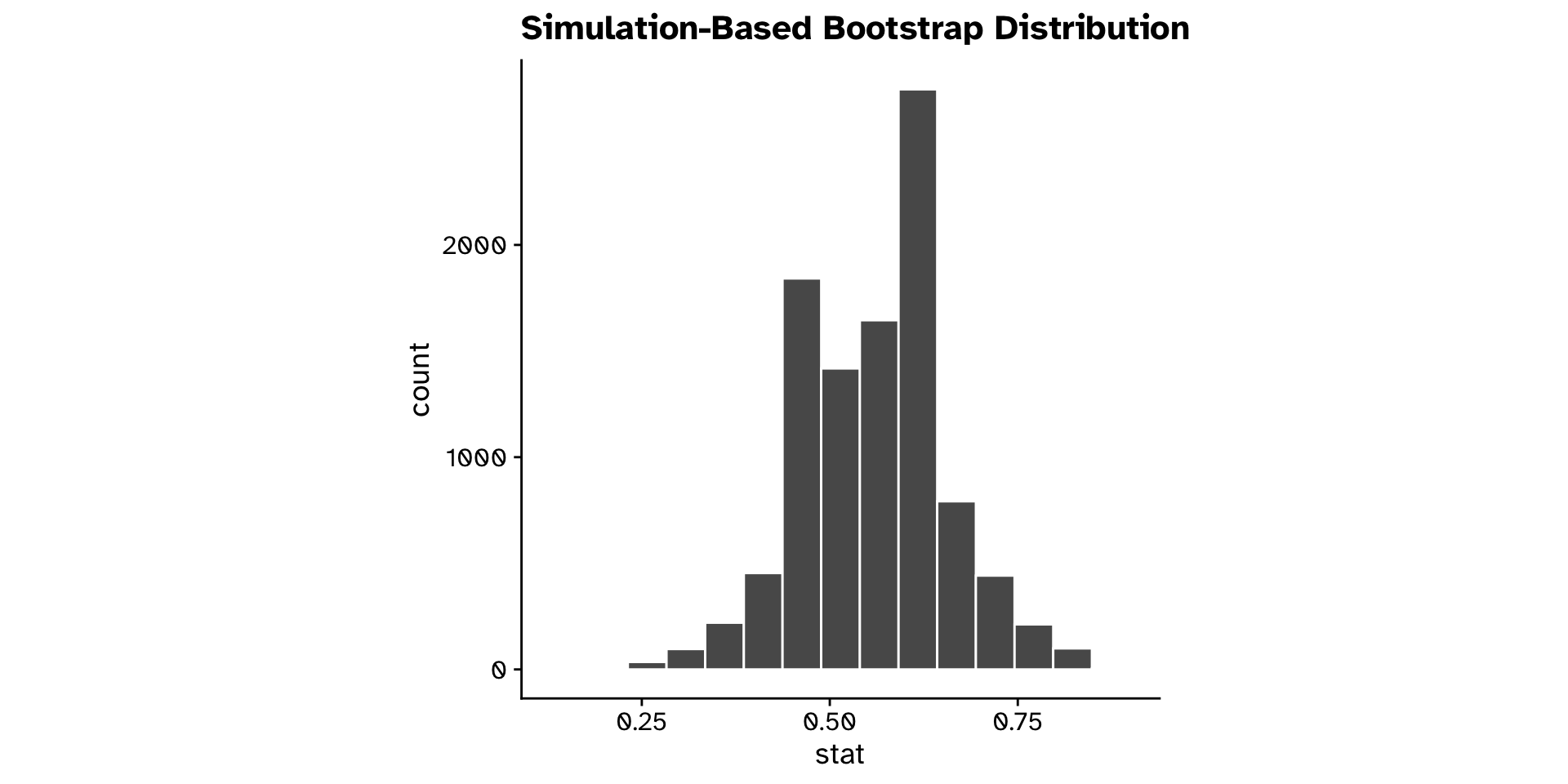
Tests of proportion
Is a proportion different from a hypothesised value? (CI)
Tests of proportion
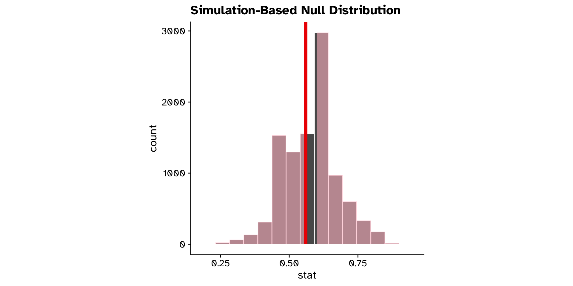
Is a proportion different from a hypothesised value? (Hyp. test)
Tests of proportion
Is a proportion different from a hypothesised value? (Hyp. test)
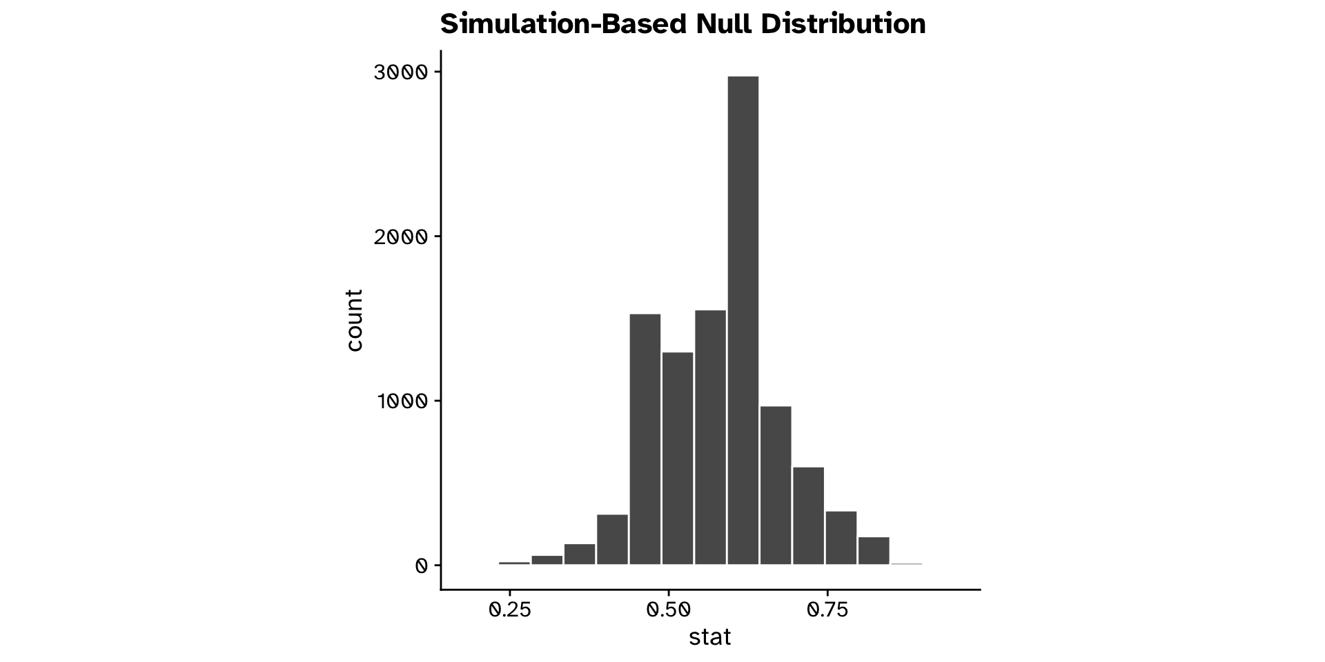
Tests of proportion
Is a proportion different from a hypothesised value? (Hyp. test)
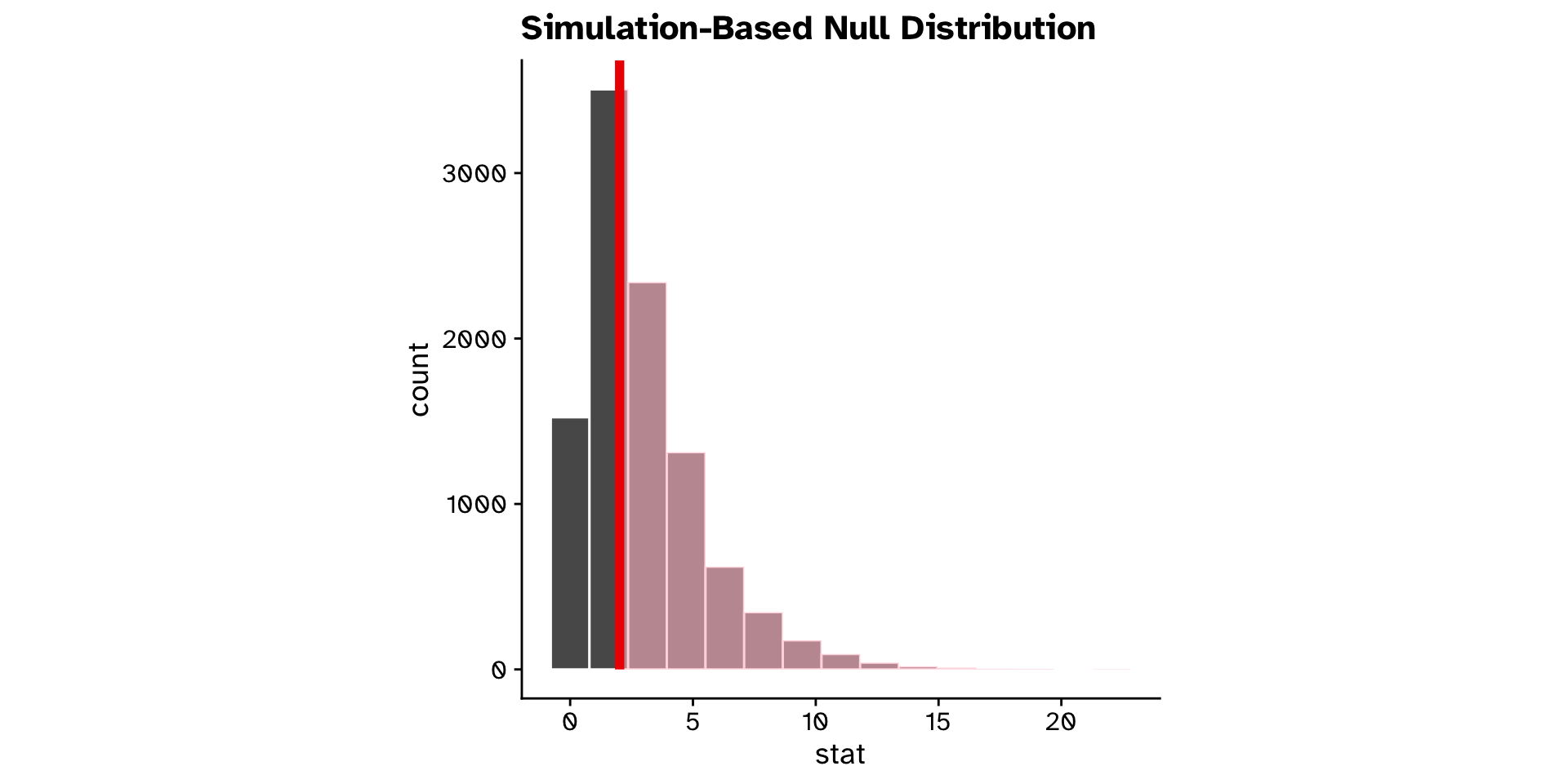
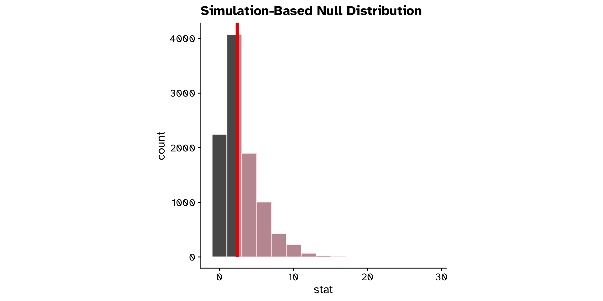
\(\chi^2\) Goodness of fit
Does the observed data differ from an expected distribution?
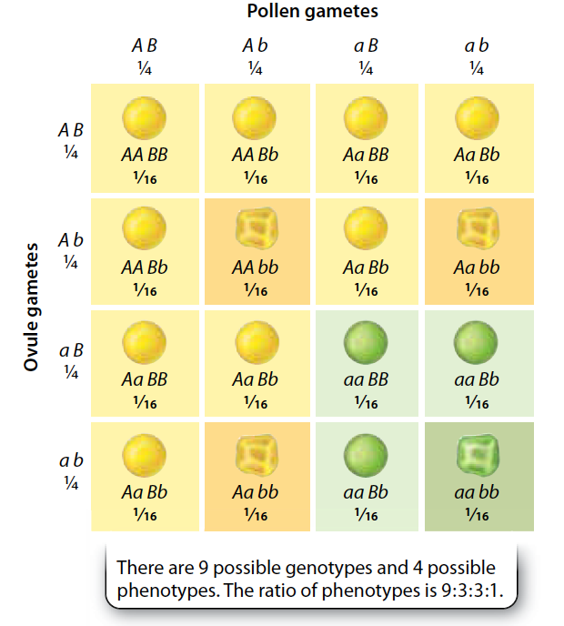
\(\chi^2\) Goodness of fit
Does the observed data differ from an expected distribution?
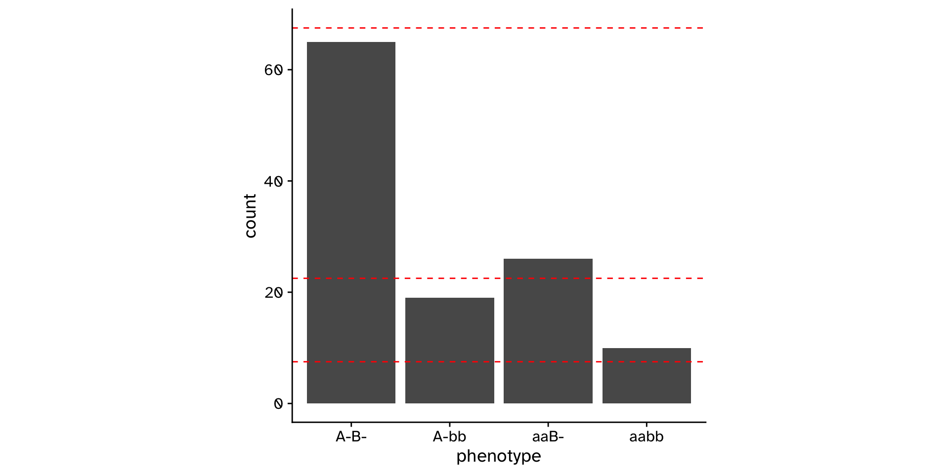
\(\chi^2\) Goodness of fit
Does the observed data differ from an expected distribution?
\(\chi^2\) Goodness of fit
Does the observed data differ from an expected distribution?
\(\chi^2\) Test of independence
Are two categorical variables associated with each other?
\(\chi^2\) Test of independence
Are two categorical variables associated with each other?
\(\chi^2\) Test of independence
Are two categorical variables associated with each other?
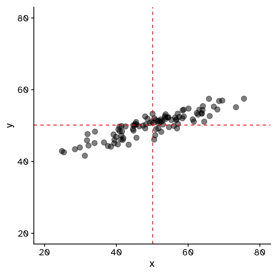
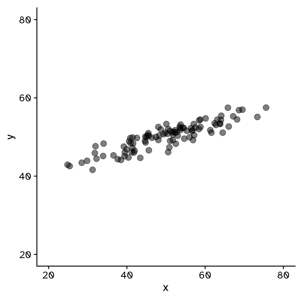
Correlation
Do two continuous variables covary?
\[ r = \frac{\text{Cov}(x,y)}{\sigma_x \sigma_y} \]

Correlation
Do two continuous variables covary?
Correlation
Do two continuous variables covary?
Correlation
Do two continuous variables covary?
Correlation
Do two continuous variables covary?
Correlation
Do two continuous variables covary?

Correlation
Do two continuous variables covary?
Correlation
Do two continuous variables covary? (CI)
Correlation
Do two continuous variables covary? (CI)
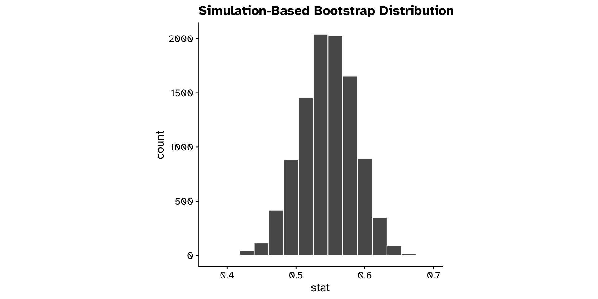
Correlation
Do two continuous variables covary? (CI)
Correlation
Do two continuous variables covary? (Hyp. test)
Correlation
Do two continuous variables covary? (Hyp. test)
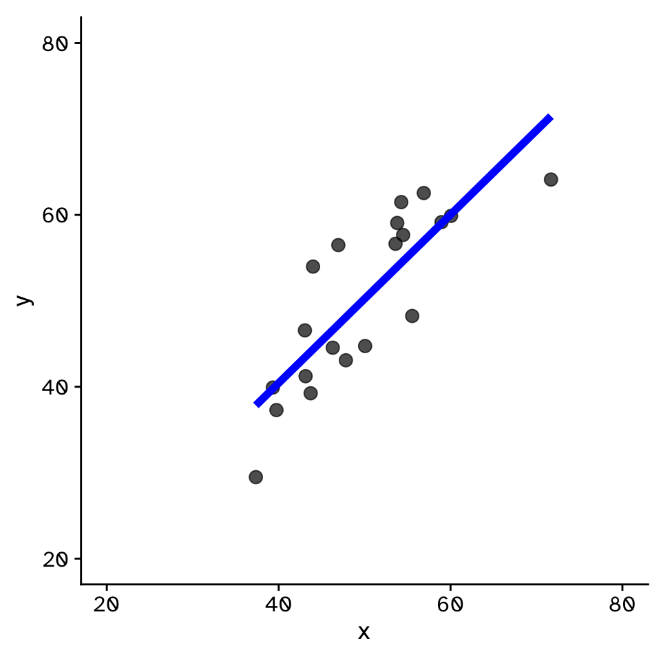
Regression
How does variable Y depend on variable X
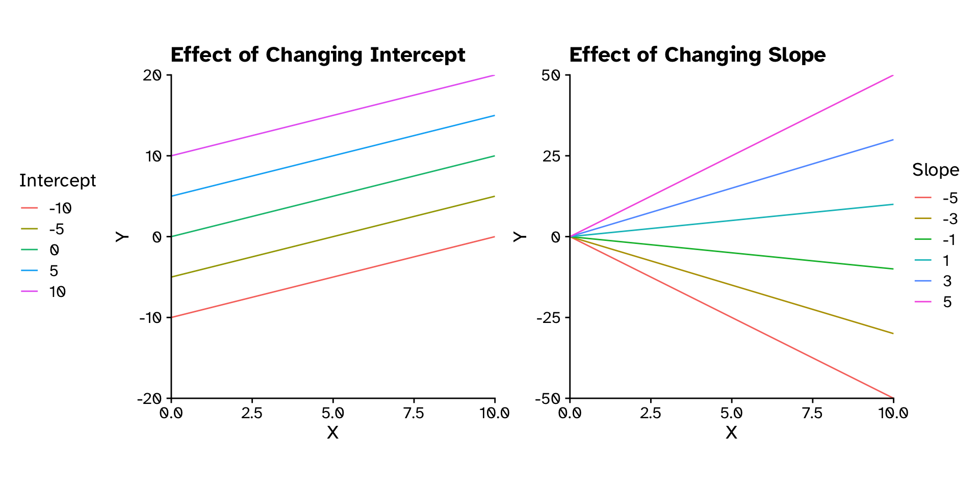
Regression
How does variable Y depend on variable X
Regression
How does variable Y depend on variable X
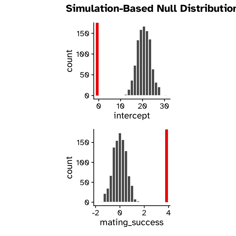
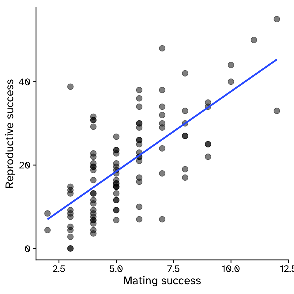
- Example: For sexual selection to operate, an increase in mating success (number of mates) must result in an increase in reproductive success (number of offspring).
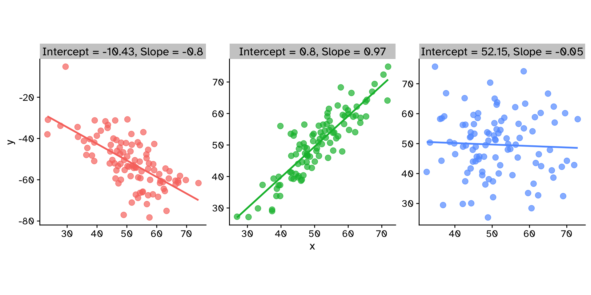
Regression
How does variable Y depend on variable X
\[ y = \beta_1x+\beta_0 \]
\[ y = 3.83x-0.68 \]
- \(\beta_1\) = strength of sexual selection
- For each additional mate, an individual (on average) gains \(\beta_1\) additional offspring
- For 5 mates (\(x=5\)):
- \(y = 3.83\times5-0.68\)
- \(y = 18.47\)

Regression
How does variable Y depend on variable X
Regression
How does variable Y depend on variable X
Regression
How does variable Y depend on variable X

Regression
How does variable Y depend on variable X
Regression
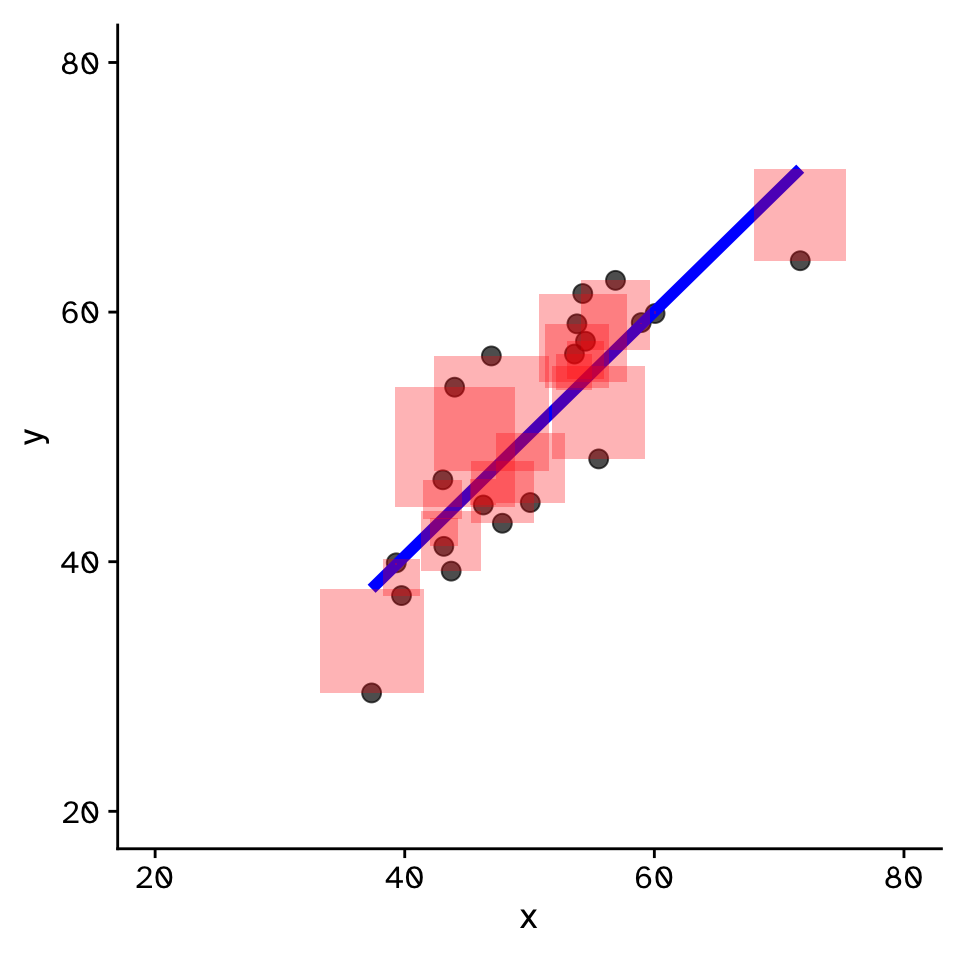
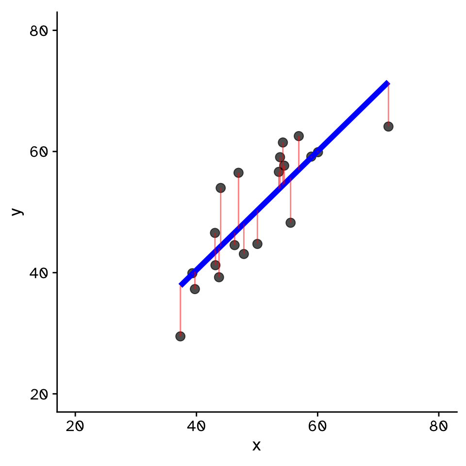
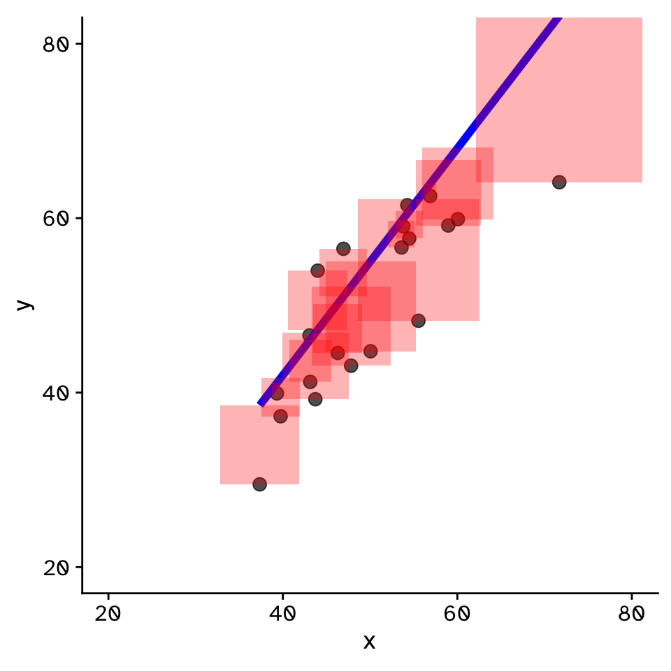
- Fit by solving to minimise the sum of the squared residuals (SSR)
- Find \(\beta_1\) and \(\beta_0\) that minimise the SSR
- Called a “loss function”
- Many approaches to do this!
How does variable Y depend on variable X
Regression
Confidence intervals
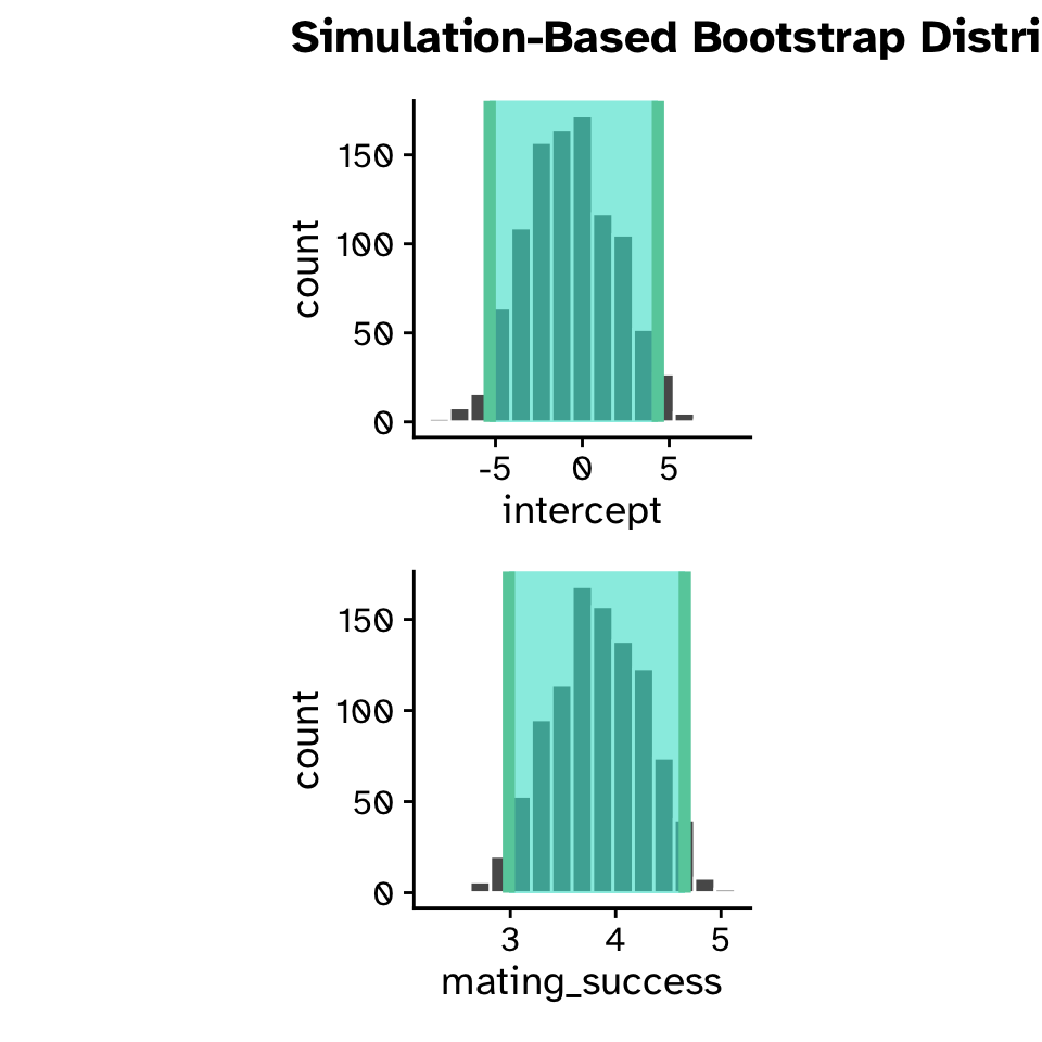
Regression
Hypothesis test