Introduction to statistical inference
Lecture 1
2026-04-27
Populations and Samples
The how and the why of statistics
- We are often limited by how much data we can collect
- We want to say something more general than the data we collect
- Example:
- Measured the species diversity in 20 spruce plantations across Sweden
- Want to say something about species diversity in all spruce plantations (in Sweden)

Populations and Samples
The how and the why of statistics
- Cannot measure species diversity in every forest in Sweden
- Instead, we collect a representative sample of data
- Use the sample to draw conclusions about the population
- Statistics allows us to approximate properties (e.g. mean species diversity) of entire populations from (usually) a single sample
Populations and Samples
The how and the why of statistics

Inference
The sampling distribution
Inference
The sampling distribution
Inference
The sampling distribution

Inference
The utility of the sampling distribution
Confidence intervals
- If we collect another sample of the same size, how much would the observed statistic vary?
Inference
The utility of the sampling distribution
Hypothesis testing
- Is our result compatible with a specific hypothesis?
Bootstrap resampling
Generating a bootstrap sampling distibution
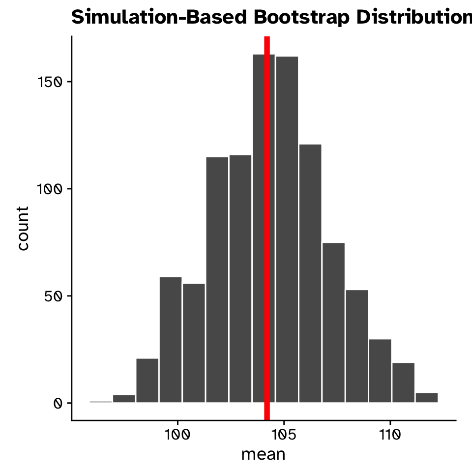
- Means from 1000 bootstrap samples
- Observed mean (mean of original sample) in red
- The observed mean is still our best guess at the true mean
- Bootstrap sampling distribution allows us to quantify our uncertainty in the mean
Bootstrap resampling
The bootstrap sampling distibution

Bootstrap resampling
Works for any statistic!
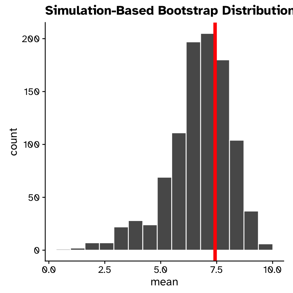
- Standard deviations from 1000 bootstrap samples
- Observed SD (SD of original sample) in red
- The observed SD is still our best guess at the true SD
- Bootstrap sampling distribution allows us to quantify our uncertainty in the SD
Bootstrap resampling
Works for any statistic!
Quantifying sampling error
The standard error (SE)
- The standard error is the standard deviation of the sampling distribution
- Use the bootstrap generated sampling distribution as our sampling distribution
- Assumptions: your sampling distribution is approximately normally distributed (bell-curve)
- If calculated with a bootstrap sampling distribution often written as \(SE_{boot}=2.7\)
Quantifying sampling error
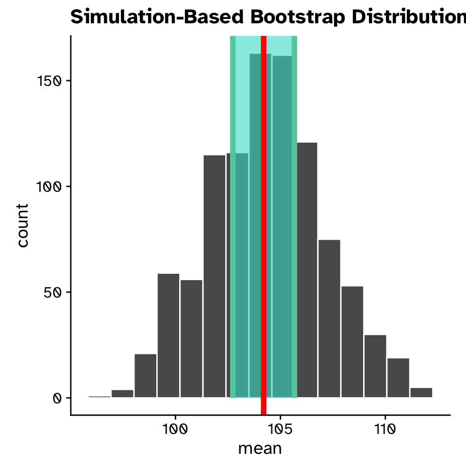
The 95% confidence interval

- If we repeated our experiment many times and calculated a 95% CI each time, the 95% CI’s would include the “true” population value 95% of the time
- Many methods to calculate:
- Percentile method: Middle 95% of the sampling distribution
- No assumptions, but requires a large (>30 >>14) sample size to be accurate
Quantifying sampling error
The 95% confidence interval
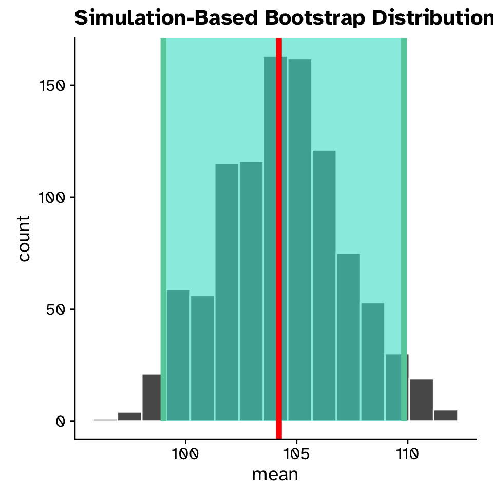
- Often reported after the observed statistic:
- Mean = 104 mm (95%CI: 99 - 110 mm)
- Less strict definition: where we expect the true population parameter to be
Confidence intervals
Using a bootstrap sampling distribution

Hypothesis testing
Back to the fish
- While watching a nature documentary, I hear that in many fish species, females are often larger than males.
- I wonder if this is true of the fish in my pond (from the previous example)?
- I hypothesise that females will be bigger than males

Hypothesis testing
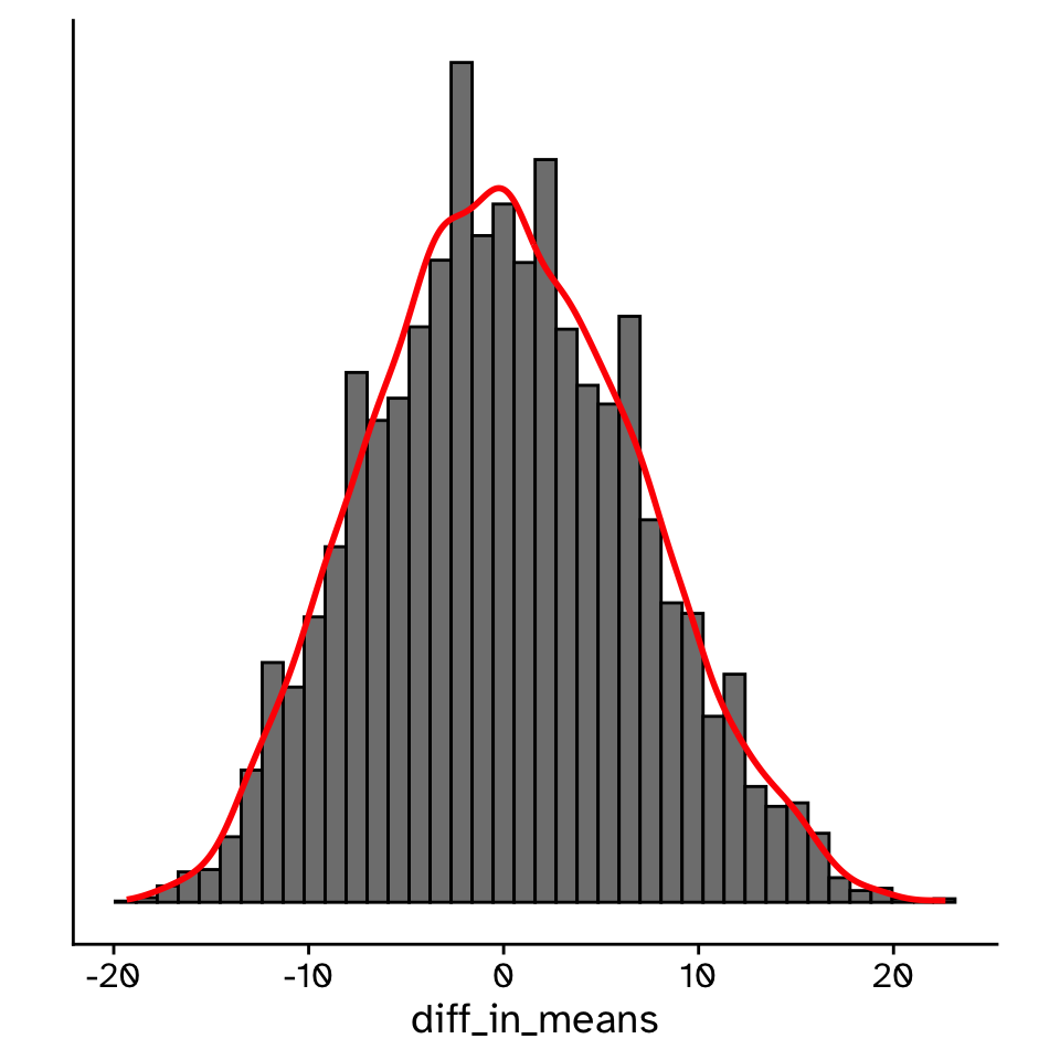
Generating a null distribution
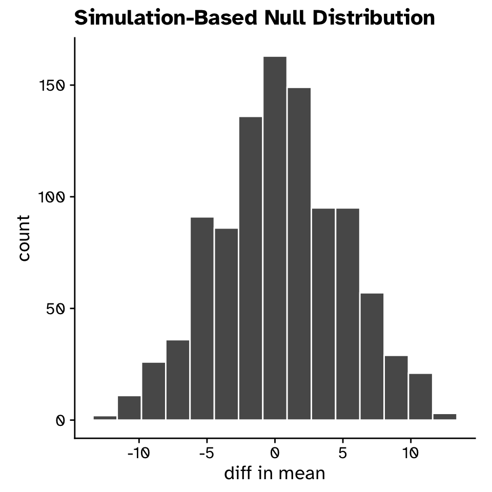
Hypothesis testing
Comparing our observed statistic against the null distribution
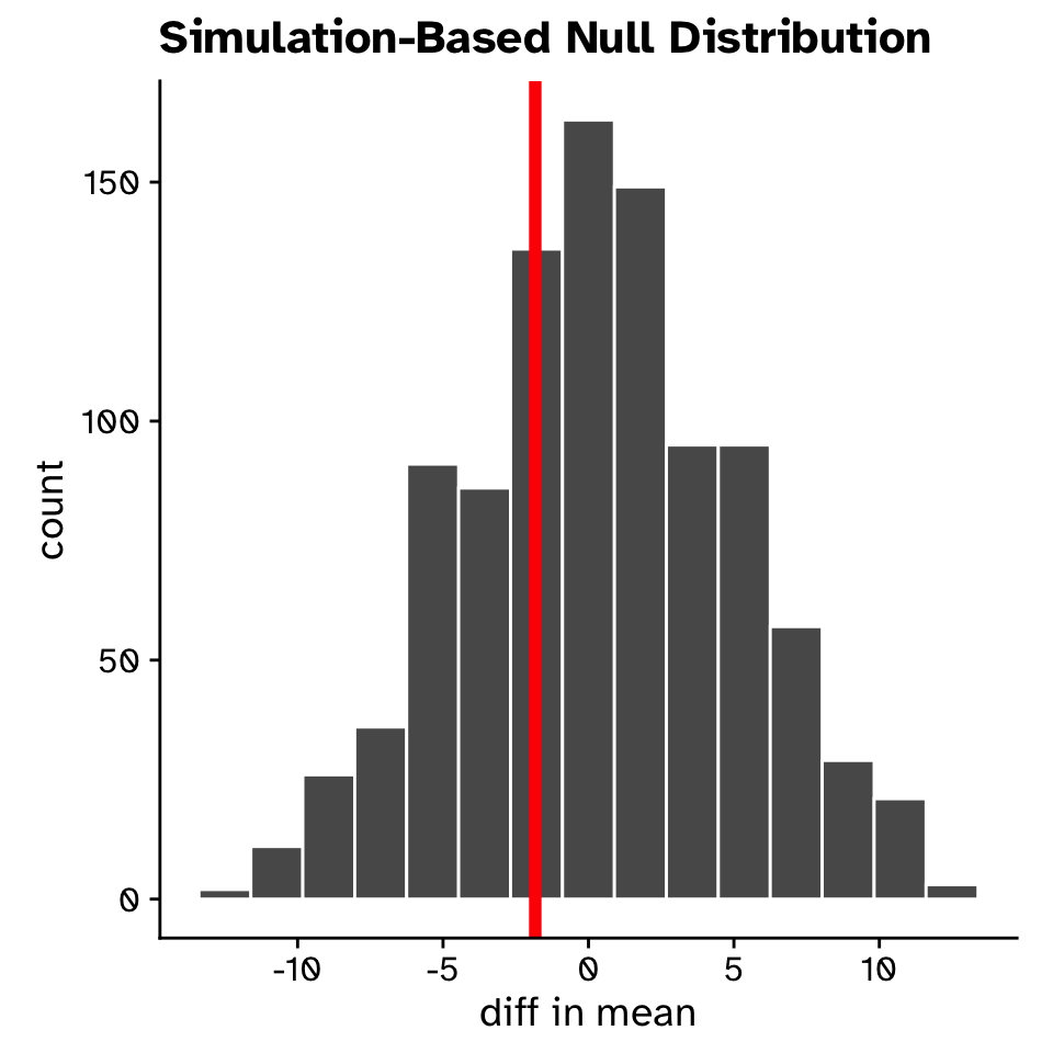
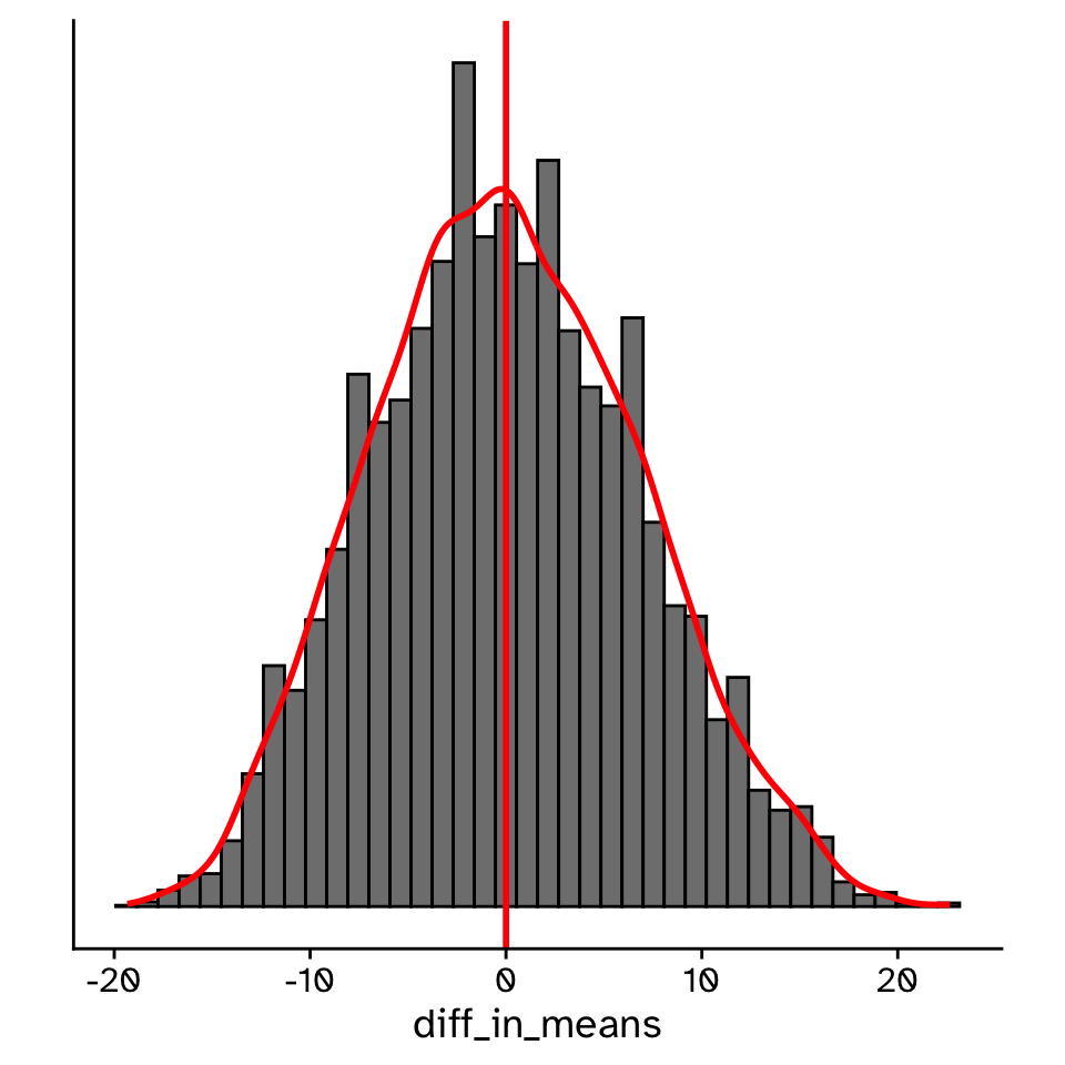
Hypothesis testing
Comparing our observed statistic against the null distribution

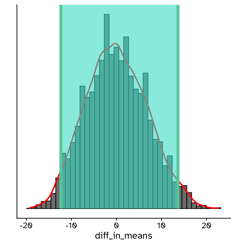
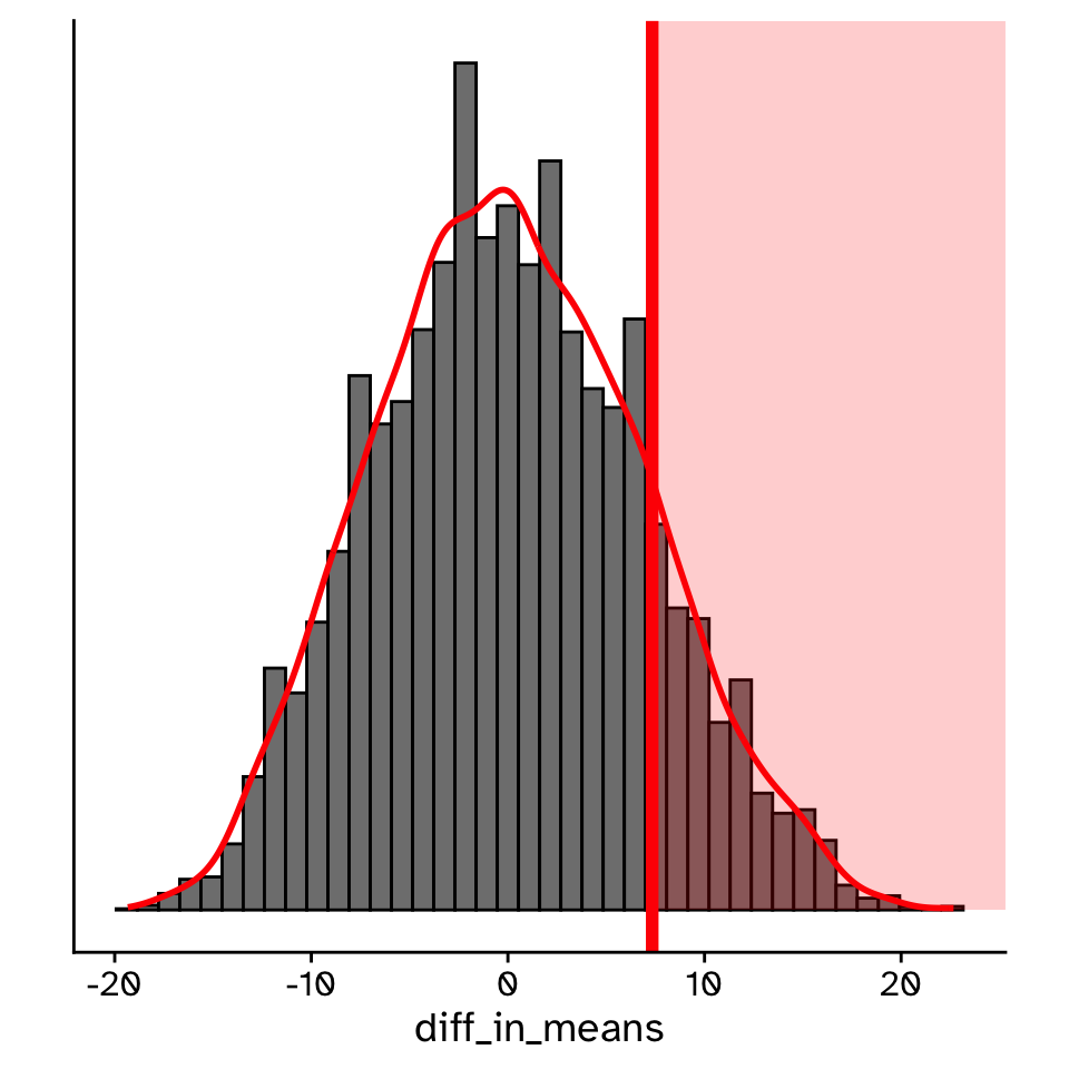
Hypothesis testing
Comparing our observed statistic against the null distribution
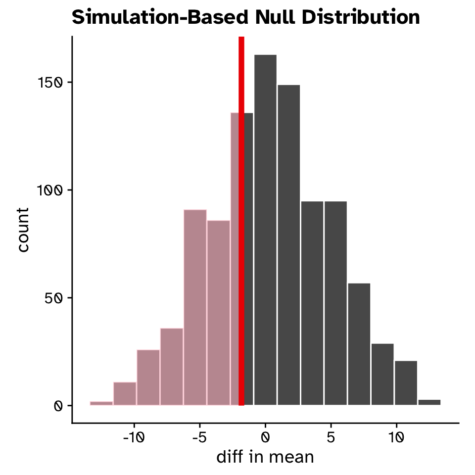
- p = 0.337
- Probability of observing our original statistic, or one more extreme, assuming the null hypothesis is true
01:30
Hypothesis testing
A framework
