I want to start sharing some of the small projects I’ve been playing around with. Most of these have come from an idea that’s popped into my head during the week, that was then written down and left on a post-it note until a rainy sunday morning came around. I get a lot more of these done in the winter, for this reason.

Anyway, about a year ago, I became fascinated with how to generate natural looking “noise” from random data. Naturally, this lead me to the work of Ken Perlin, and to what is known as Perlin noise. One of the first rainy morning projects that stemmed from this interest, was to try and generate random island maps.

For this project, I am using R, along with the package {ambient}, which is a wrapper for the FastNoise C++ library. In the future, I will tidy up and publish my attempt at writing a Perlin noise generator in R directly. For this post though, we will use {ambient} to generate our noise.

The basic idea

This idea is simple and far from unique:

Generate some Perlin noise.
Multiple that noise by a kernal to create a bias in the centre of the map.
Colour the resulting height map to look like a map.

Generating some Perlin noise

Here I use the noise_perlin() function to generate a matrix of Perlin noise values, pn, with dimensions map_dim, using n_oct octaves. Having n_oct > 1 means adding a fractal nature to the noise. Essentially, the same process is repeated to generate the Perlin noise, but at a higher detail level, but with reduced amplitude, and then added to our original Perlin noise. I then normalise() the values to be between 0 and 1.

Code

library(ambient)

map_dim <- c(300, 300)
n_oct <- 6

set.seed(1478914098)

pn <- noise_perlin(dim = map_dim, octaves = n_oct) |> normalise()

We can plot our output to see how it’s looking:

Code

par(mar = rep(0.025, 4))
plot(as.raster(pn))

Yep, that’s some Perlin noise. Dark regions will become oceans, and lighter regions will be come land and mountains. This effect becomes much more obvious with some recolouring, so I will do that now, before we go to step 2.

Adding some basic colour

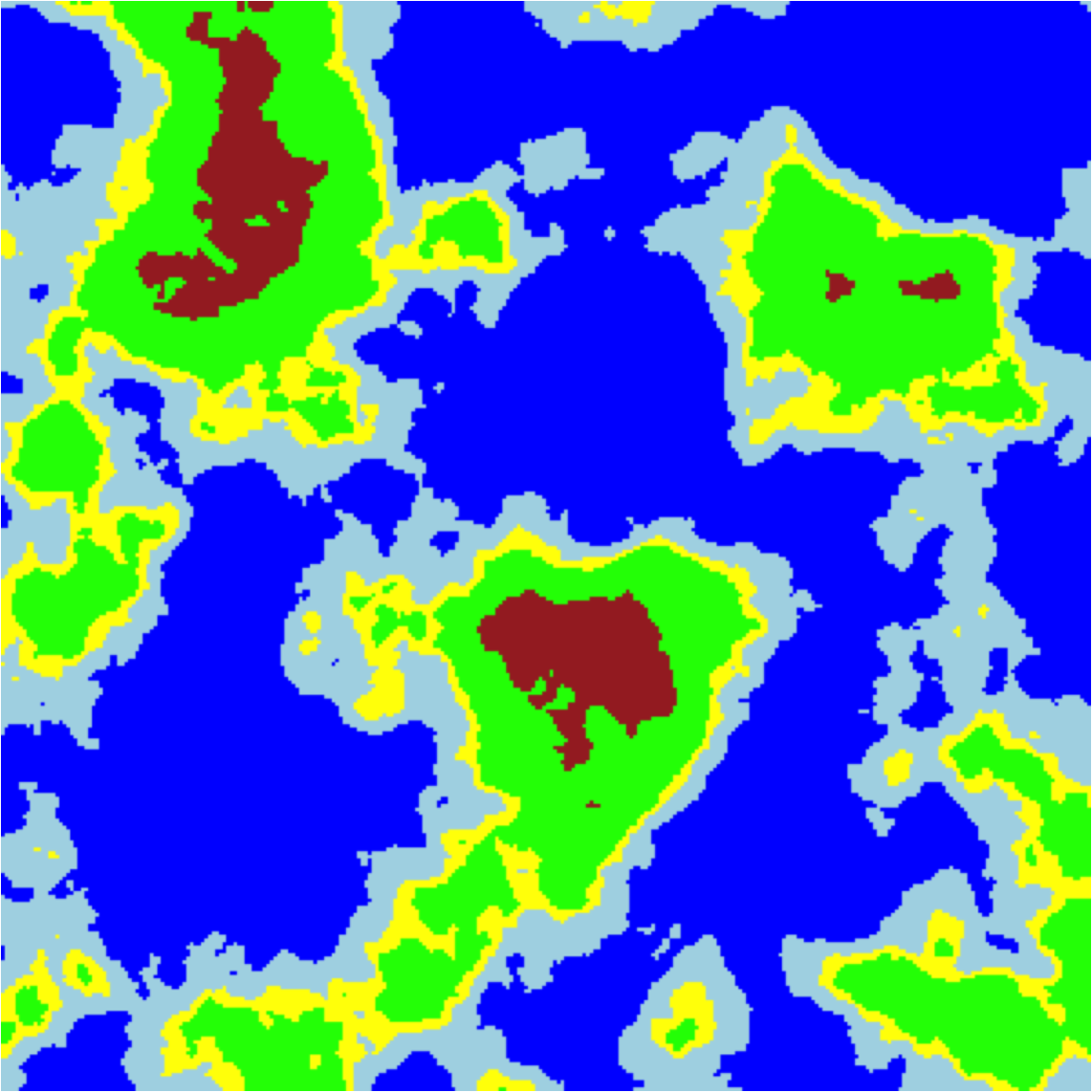
First I will define the cut off boundry points for each of my types of terrain, and an associated colour. We then loop through all values in the pn matrix, and assign them a colour, and save that in pn_col

Code

col_data <-
  list(
    deep_water = list(0.40, "blue"),
    shallow_water = list(0.5, "lightblue"),
    sand = list(0.55, "yellow"),
    grass = list(0.8, "green"),
    mountain = list(1, "brown")
  )

colour_noise <- function(pn, col_data) {
  pn_col <- matrix(NA, nrow = nrow(pn), ncol = ncol(pn))
  
  for (i in 1:nrow(pn)) {
    for (j in 1:ncol(pn)) {
      value <- pn[i, j]
      if (value <= col_data$deep_water[[1]]) {
        pn_col[i, j] <- col_data$deep_water[[2]]
      } else if (value <= col_data$shallow_water[[1]]) {
        pn_col[i, j] <- col_data$shallow_water[[2]]
      } else if (value <= col_data$sand[[1]]) {
        pn_col[i, j] <- col_data$sand[[2]]
      } else if (value <= col_data$grass[[1]]) {
        pn_col[i, j] <- col_data$grass[[2]]
      } else {
        pn_col[i, j] <- col_data$mountain[[2]]
      }
    }
  }
  
  return(pn_col)
}

pn_col <- colour_noise(pn, col_data)

par(mar = rep(0.025, 4))
plot(as.raster(pn_col))

Now that looks more like a map.

Creating a bias towards a central island

I think the easiest way to to this, is to multiple pn by some sort of kernal. I will use a gaussian one for this:

Code

gaussian_kernel <- function(size, sigma) {
  center <- (size - 1) / 2
  kernel <- outer(
    0:(size - 1), 0:(size - 1),
    function(x, y) exp(-((x - center)^2 + (y - center)^2) / (2 * sigma^2))
  )
  kernel / sum(kernel)
}

island_bias <- gaussian_kernel(map_dim[1], map_dim[1]/2) |> normalise()

par(mar = rep(0.025, 4))
plot(as.raster(island_bias))

Which I then multiple with pn and colourise to give:

Code

pn_bias <- pn*island_bias

par(mar = rep(0.025, 4))
plot(as.raster(colour_noise(pn_bias, col_data)))

Some fancier colour

Next, I will add some nicer colouration to the map. I add a colour gradient for each terrain type:

Code

terrain_pal <- list(
  deep_water = list(
    range = c(0, 0.4),
    pal = c("#4357b3", "#5c7aff"),
    bias = 10
  ),
  shallow_water = list(
    range = c(0.4, 0.5),
    pal = c("#90d9f1", "#e9faff"),
    bias = 0.001
  ),
  sand = list(
    range = c(0.5, 0.52),
    pal = c("#FFEF9F", "#FFEF9F"),
    bias = 1
  ),
  grass = list(
    range = c(0.52, 0.8),
    pal = c("#4f772d", "#90a955", "#EDD6AB"),
    bias = 0.1
  ),
  mountain = list(
    range = c(0.8, 1),
    pal = c("#a9927d", "#5e503f", "white"),
    bias = 1
  )
)

map_pal <- 
  lapply(
    terrain_pal, 
    function(i) {
      ramp_func <- colorRampPalette(i$pal, bias = i$bias)
      ramp_func((i$range[[2]]-i$range[[1]])/10^(-2))
    }
  ) |> unlist()

names(map_pal) <- seq(0, 1, 10^(-2))


pn_bias_round <- round(pn_bias, 2)

pn_bias_col <- matrix(NA, nrow = nrow(pn_bias_round), ncol = ncol(pn_bias_round))

for (i in 1:nrow(pn_bias_round)) {
  for (j in 1:ncol(pn_bias_round)) {
    pn_bias_col[i, j] <- map_pal[paste0(pn_bias_round[i, j])]
  }
}

par(mar = rep(0.025, 4))
plot(as.raster(pn_bias_col))

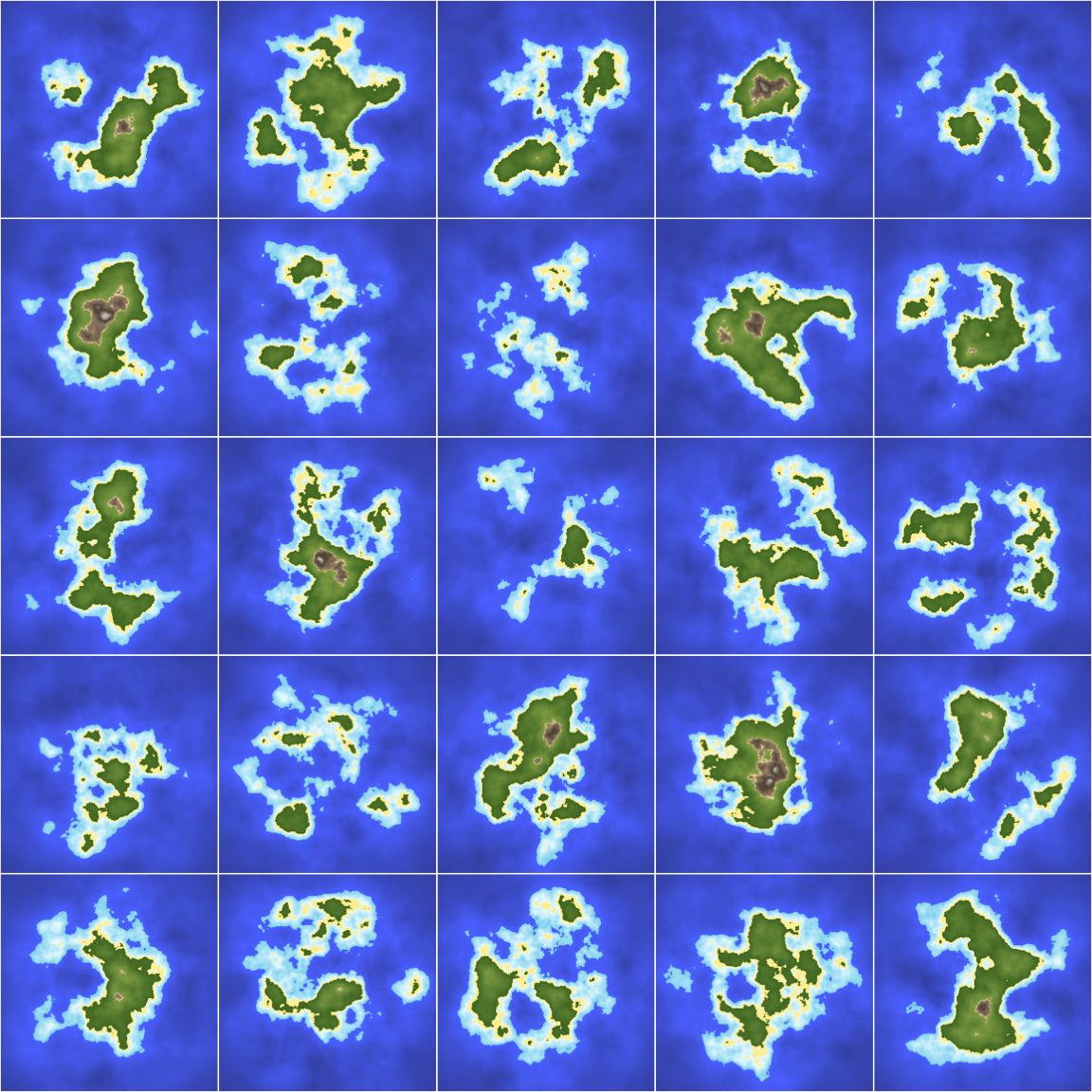
Finally, I will tidy this up, wrap it all into a single function, and generate a set of maps:

Code

gen_map <- function(map_dim = c(300, 300), n_oct = 6, palette, col_detail = 2) {

  pn <- noise_perlin(dim = map_dim, octaves = n_oct) |> normalise()
  island_bias <- gaussian_kernel(map_dim[1], map_dim[1]/2) |> normalise()
  pn_biased <- pn * island_bias

  map_pal <- 
    lapply(
      palette, 
      function(i) {
        ramp_func <- colorRampPalette(i$pal, bias = i$bias)
        ramp_func((i$range[[2]]-i$range[[1]])/10^(-col_detail))
      }
    ) |> unlist()

  names(map_pal) <- seq(0, 1, 10^(-col_detail))

  pn_biased_round <- round(pn_biased, col_detail)

  pn_biased_col <- matrix(NA, nrow = nrow(pn_biased_round), ncol = ncol(pn_biased_round))

  for (i in 1:nrow(pn_biased_round)) {
    for (j in 1:ncol(pn_biased_round)) {
      pn_biased_col[i, j] <- map_pal[paste0(pn_biased_round[i, j])]
    }
  }

  plot(as.raster(pn_biased_col))

}

par(mfrow = c(5, 5), mar = rep(0.025, 4))

for (i in 1:25) {
  gen_map(palette = terrain_pal)
}

I find it endlessly fun just generating random maps this way. I think it hits at my nostalgia for early 2000s RTS games. I might try and turn this into a webR or shiny app some day. Until then, if you want to play around with it, you can download the .qmd file from the code link at the top of the page.

That’s all!

sessionInfo()

R version 4.4.1 (2024-06-14)
Platform: aarch64-apple-darwin20
Running under: macOS Sonoma 14.5

Matrix products: default
BLAS:   /Library/Frameworks/R.framework/Versions/4.4-arm64/Resources/lib/libRblas.0.dylib 
LAPACK: /Library/Frameworks/R.framework/Versions/4.4-arm64/Resources/lib/libRlapack.dylib;  LAPACK version 3.12.0

locale:
[1] en_US.UTF-8/en_US.UTF-8/en_US.UTF-8/C/en_US.UTF-8/en_US.UTF-8

time zone: Europe/Stockholm
tzcode source: internal

attached base packages:
[1] stats     graphics  grDevices utils     datasets  methods   base     

other attached packages:
[1] ambient_1.0.2

loaded via a namespace (and not attached):
 [1] htmlwidgets_1.6.4 compiler_4.4.1    fastmap_1.2.0     cli_3.6.3        
 [5] tools_4.4.1       htmltools_0.5.8.1 yaml_2.3.10       rmarkdown_2.28   
 [9] knitr_1.48        jsonlite_1.8.9    xfun_0.48         digest_0.6.37    
[13] rlang_1.1.4       evaluate_1.0.1

--- title: "Perlin islands" author: "Iain R. Moodie" date: 2024-10-27 categories: [R, just-for-fun] draft: false format: html: code-fold: true code-tools: true code-overflow: wrap execute: echo: true warning: false eval: true output-format: png dpi: 96 fig-width: 6 fig-height: 6 --- I want to start sharing some of the small projects I've been playing around with. Most of these have come from an idea that's popped into my head during the week, that was then written down and left on a post-it note until a rainy sunday morning came around. I get a lot more of these done in the winter, for this reason. Anyway, about a year ago, I became fascinated with how to generate natural looking "noise" from random data. Naturally, this lead me to the work of [Ken Perlin](https://en.wikipedia.org/wiki/Ken_Perlin), and to what is known as [Perlin noise](https://en.wikipedia.org/wiki/Perlin_noise). One of the first rainy morning projects that stemmed from this interest, was to try and generate random island maps. For this project, I am using `R`, along with the package [`{ambient}`](https://ambient.data-imaginist.com/), which is a wrapper for the [FastNoise](https://github.com/Auburn/FastNoiseLite) `C++` library. In the future, I will tidy up and publish my attempt at writing a Perlin noise generator in `R` directly. For this post though, we will use `{ambient}` to generate our noise. # The basic idea This idea is simple and far from unique: 1. Generate some Perlin noise. 2. Multiple that noise by a kernal to create a bias in the centre of the map. 3. Colour the resulting height map to look like a map. # Generating some Perlin noise Here I use the `noise_perlin()` function to generate a matrix of Perlin noise values, `pn`, with dimensions `map_dim`, using `n_oct` octaves. Having `n_oct` > 1 means adding a fractal nature to the noise. Essentially, the same process is repeated to generate the Perlin noise, but at a higher detail level, but with reduced amplitude, and then added to our original Perlin noise. I then `normalise()` the values to be between 0 and 1. ```{r, gen_pn} library(ambient) map_dim <- c(300, 300) n_oct <- 6 set.seed(1478914098) pn <- noise_perlin(dim = map_dim, octaves = n_oct) |> normalise() ``` We can plot our output to see how it's looking: ```{r, plot_pn} #| fig-align: center par(mar = rep(0.025, 4)) plot(as.raster(pn)) ``` Yep, that's some Perlin noise. Dark regions will become oceans, and lighter regions will be come land and mountains. This effect becomes much more obvious with some recolouring, so I will do that now, before we go to step 2. # Adding some basic colour First I will define the cut off boundry points for each of my types of terrain, and an associated colour. We then loop through all values in the `pn` matrix, and assign them a colour, and save that in `pn_col` ```{r, col_noise} #| fig-align: center col_data <- list( deep_water = list(0.40, "blue"), shallow_water = list(0.5, "lightblue"), sand = list(0.55, "yellow"), grass = list(0.8, "green"), mountain = list(1, "brown") ) colour_noise <- function(pn, col_data) { pn_col <- matrix(NA, nrow = nrow(pn), ncol = ncol(pn)) for (i in 1:nrow(pn)) { for (j in 1:ncol(pn)) { value <- pn[i, j] if (value <= col_data$deep_water[[1]]) { pn_col[i, j] <- col_data$deep_water[[2]] } else if (value <= col_data$shallow_water[[1]]) { pn_col[i, j] <- col_data$shallow_water[[2]] } else if (value <= col_data$sand[[1]]) { pn_col[i, j] <- col_data$sand[[2]] } else if (value <= col_data$grass[[1]]) { pn_col[i, j] <- col_data$grass[[2]] } else { pn_col[i, j] <- col_data$mountain[[2]] } } } return(pn_col) } pn_col <- colour_noise(pn, col_data) par(mar = rep(0.025, 4)) plot(as.raster(pn_col)) ``` Now that looks more like a map. # Creating a bias towards a central island I think the easiest way to to this, is to multiple `pn` by some sort of kernal. I will use a gaussian one for this: ```{r, island_bias} #| fig-align: center gaussian_kernel <- function(size, sigma) { center <- (size - 1) / 2 kernel <- outer( 0:(size - 1), 0:(size - 1), function(x, y) exp(-((x - center)^2 + (y - center)^2) / (2 * sigma^2)) ) kernel / sum(kernel) } island_bias <- gaussian_kernel(map_dim[1], map_dim[1]/2) |> normalise() par(mar = rep(0.025, 4)) plot(as.raster(island_bias)) ``` Which I then multiple with `pn` and colourise to give: ```{r, pn_island} #| fig-align: center pn_bias <- pn*island_bias par(mar = rep(0.025, 4)) plot(as.raster(colour_noise(pn_bias, col_data))) ``` # Some fancier colour Next, I will add some nicer colouration to the map. I add a colour gradient for each terrain type: ```{r} #| fig-align: center #| classes: preview-image terrain_pal <- list( deep_water = list( range = c(0, 0.4), pal = c("#4357b3", "#5c7aff"), bias = 10 ), shallow_water = list( range = c(0.4, 0.5), pal = c("#90d9f1", "#e9faff"), bias = 0.001 ), sand = list( range = c(0.5, 0.52), pal = c("#FFEF9F", "#FFEF9F"), bias = 1 ), grass = list( range = c(0.52, 0.8), pal = c("#4f772d", "#90a955", "#EDD6AB"), bias = 0.1 ), mountain = list( range = c(0.8, 1), pal = c("#a9927d", "#5e503f", "white"), bias = 1 ) ) map_pal <- lapply( terrain_pal, function(i) { ramp_func <- colorRampPalette(i$pal, bias = i$bias) ramp_func((i$range[[2]]-i$range[[1]])/10^(-2)) } ) |> unlist() names(map_pal) <- seq(0, 1, 10^(-2)) pn_bias_round <- round(pn_bias, 2) pn_bias_col <- matrix(NA, nrow = nrow(pn_bias_round), ncol = ncol(pn_bias_round)) for (i in 1:nrow(pn_bias_round)) { for (j in 1:ncol(pn_bias_round)) { pn_bias_col[i, j] <- map_pal[paste0(pn_bias_round[i, j])] } } par(mar = rep(0.025, 4)) plot(as.raster(pn_bias_col)) ``` Finally, I will tidy this up, wrap it all into a single function, and generate a set of maps: ```{r} #| fig-align: center gen_map <- function(map_dim = c(300, 300), n_oct = 6, palette, col_detail = 2) { pn <- noise_perlin(dim = map_dim, octaves = n_oct) |> normalise() island_bias <- gaussian_kernel(map_dim[1], map_dim[1]/2) |> normalise() pn_biased <- pn * island_bias map_pal <- lapply( palette, function(i) { ramp_func <- colorRampPalette(i$pal, bias = i$bias) ramp_func((i$range[[2]]-i$range[[1]])/10^(-col_detail)) } ) |> unlist() names(map_pal) <- seq(0, 1, 10^(-col_detail)) pn_biased_round <- round(pn_biased, col_detail) pn_biased_col <- matrix(NA, nrow = nrow(pn_biased_round), ncol = ncol(pn_biased_round)) for (i in 1:nrow(pn_biased_round)) { for (j in 1:ncol(pn_biased_round)) { pn_biased_col[i, j] <- map_pal[paste0(pn_biased_round[i, j])] } } plot(as.raster(pn_biased_col)) } par(mfrow = c(5, 5), mar = rep(0.025, 4)) for (i in 1:25) { gen_map(palette = terrain_pal) } ``` I find it endlessly fun just generating random maps this way. I think it hits at my nostalgia for early 2000s RTS games. I might try and turn this into a `webR` or `shiny` app some day. Until then, if you want to play around with it, you can download the `.qmd` file from the code link at the top of the page. That's all! ```{r} #| code-fold: false sessionInfo() ```