Load packages
library (infer)library (tidyverse)
── Attaching core tidyverse packages ──────────────────────── tidyverse 2.0.0 ──
✔ dplyr     1.2.0     ✔ readr     2.2.0
✔ forcats   1.0.1     ✔ stringr   1.6.0
✔ ggplot2   4.0.2     ✔ tibble    3.3.1
✔ lubridate 1.9.5     ✔ tidyr     1.3.2
✔ purrr     1.2.1
── Conflicts ────────────────────────────────────────── tidyverse_conflicts() ──
✖ dplyr::filter() masks stats::filter()
✖ dplyr::lag()    masks stats::lag()
ℹ Use the conflicted package (<http://conflicted.r-lib.org/>) to force all conflicts to become errors
theme_set (theme_bw (base_size = 16 ) + theme (aspect.ratio = 1 )) # sets a global ggplot2 theme
Generate fake data
set.seed (11 )<- paste0 ("sp_" , 1 : 7 )<- tibble (environment = rep (c ("env_a" , "env_b" ), each = 7 ),species = rep (species_levels, times = 2 ),n = c (18 , 14 , 12 , 10 , 9 , 8 , 0 , # env_a 45 , 9 , 11 , 13 , 15 , 17 , 19 # env_b |> :: uncount (n)
# A tibble: 200 × 2
   environment species
   <chr>       <chr>
 1 env_a       sp_1
 2 env_a       sp_1
 3 env_a       sp_1
 4 env_a       sp_1
 5 env_a       sp_1
 6 env_a       sp_1
 7 env_a       sp_1
 8 env_a       sp_1
 9 env_a       sp_1
10 env_a       sp_1
# ℹ 190 more rows
Shannon diversity index
Shannon diversity index function for use with infer::calculate(). Copy this function into your document and run it so that you can use with later.
<- function (x, order, ...) {<- x$ species<- table (species) / length (species)if (length (props) == 1 ) {return (0 )# Only sum over non-zero proportions to avoid log(0) <- - sum (props[props > 0 ] * log (props[props > 0 ]))
Calculate observed
<- |> filter (environment == "env_a" ) |> specify (response = species) |> calculate (stat = stat_shannon)<- |> filter (environment == "env_b" ) |> specify (response = species) |> calculate (stat = stat_shannon)
Boostrap sampling distribution
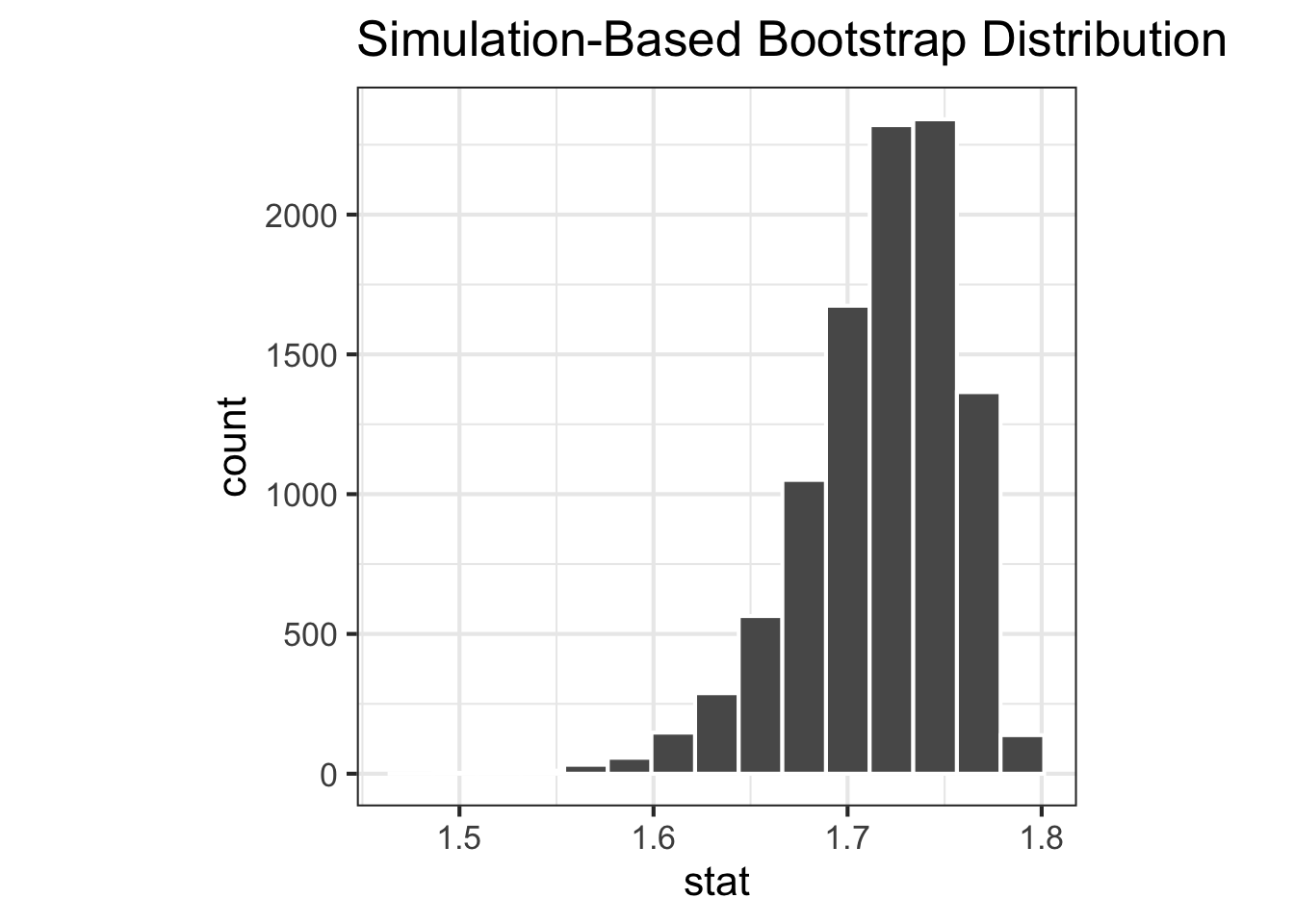
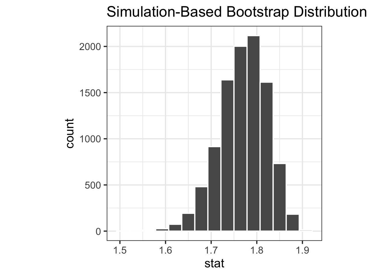
<- |> filter (environment == "env_a" ) |> specify (response = species) |> generate (reps = 10000 , type = "bootstrap" ) |> calculate (stat = stat_shannon)<- |> filter (environment == "env_b" ) |> specify (response = species) |> generate (reps = 10000 , type = "bootstrap" ) |> calculate (stat = stat_shannon)|> visualise ()
Confidence interval
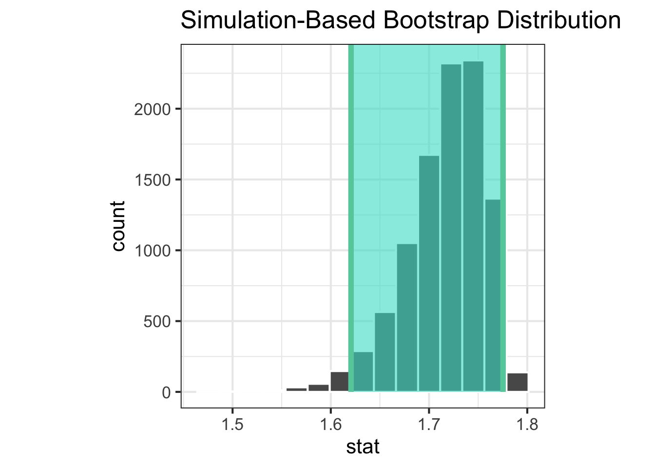
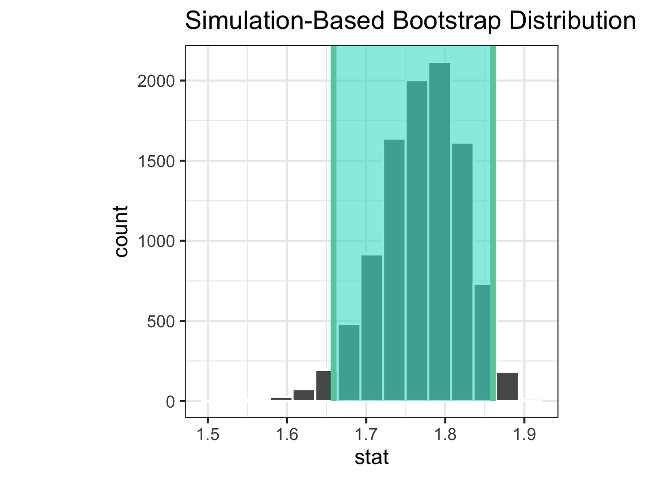
<- |> get_ci (level = 0.95 , type = "percentile" )<- |> get_ci (level = 0.95 , type = "percentile" )
# A tibble: 1 × 2
  lower_ci upper_ci
     <dbl>    <dbl>
1     1.62     1.78
# A tibble: 1 × 2
  lower_ci upper_ci
     <dbl>    <dbl>
1     1.66     1.86
|> visualise () + shade_ci (endpoints = ci_a)|> visualise () + shade_ci (endpoints = ci_b)
Plots
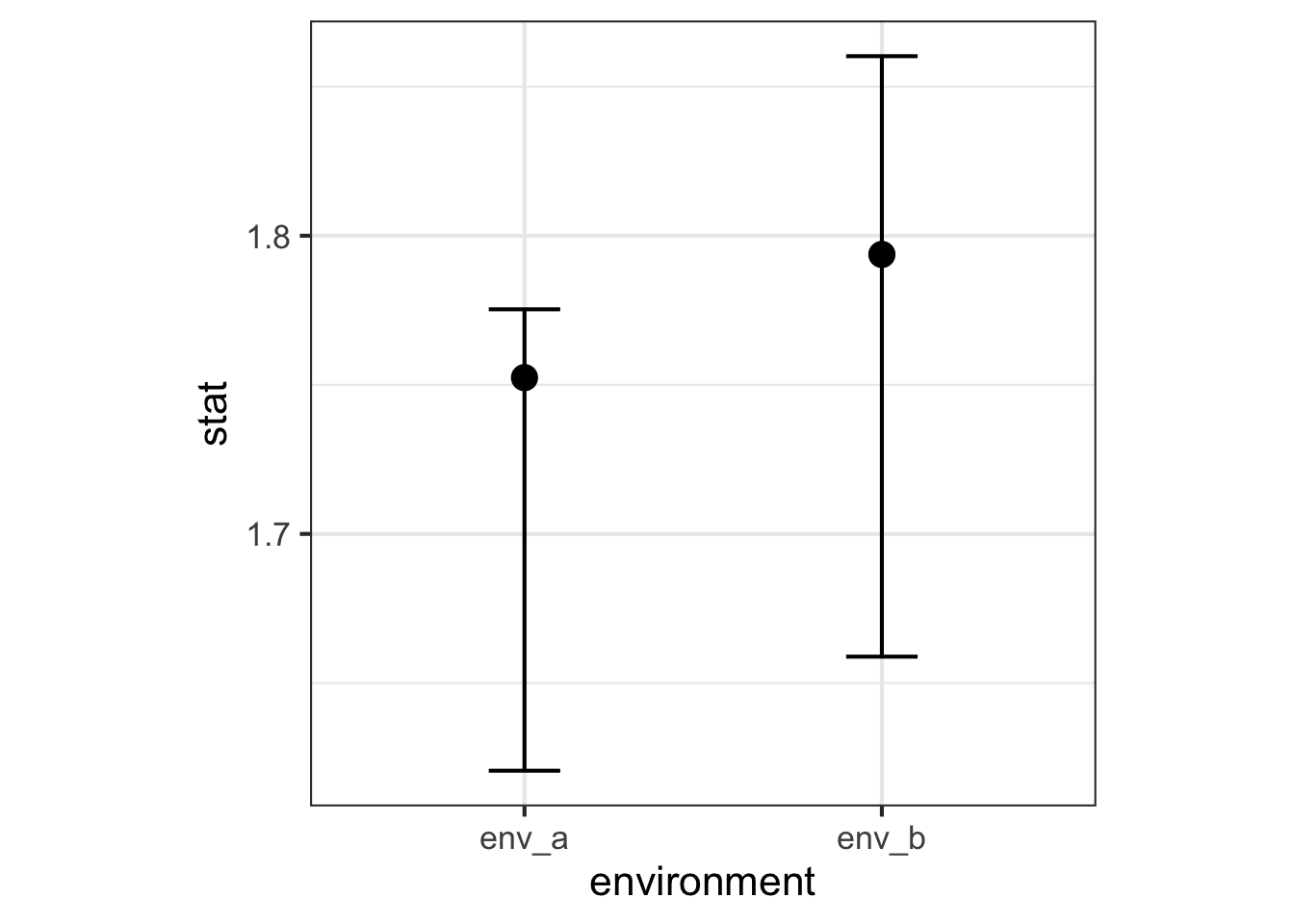
<- bind_rows (env_a = obs_a,env_b = obs_b,.id = "environment" <- bind_rows (env_a = ci_a,env_b = ci_b,.id = "environment" |> full_join (ci_shannon, by = join_by (environment)) |> ggplot (aes (x = environment, y = stat)) + geom_point (size = 4 ) + geom_errorbar (aes (ymin = lower_ci, ymax = upper_ci), width = 0.2 )
Simpson diversity index
Simpson diversity index function for use with infer::calculate(). Copy this function into your document and run it so that you can use with later.
<- function (x, order, ...) {<- x$ species<- table (species) / length (species)# Simpson index: 1 - sum(p_i^2) <- 1 - sum (props^ 2 )
Calculate observed
<- |> filter (environment == "env_a" ) |> specify (response = species) |> calculate (stat = stat_simpson)<- |> filter (environment == "env_b" ) |> specify (response = species) |> calculate (stat = stat_simpson)
Boostrap sampling distribution
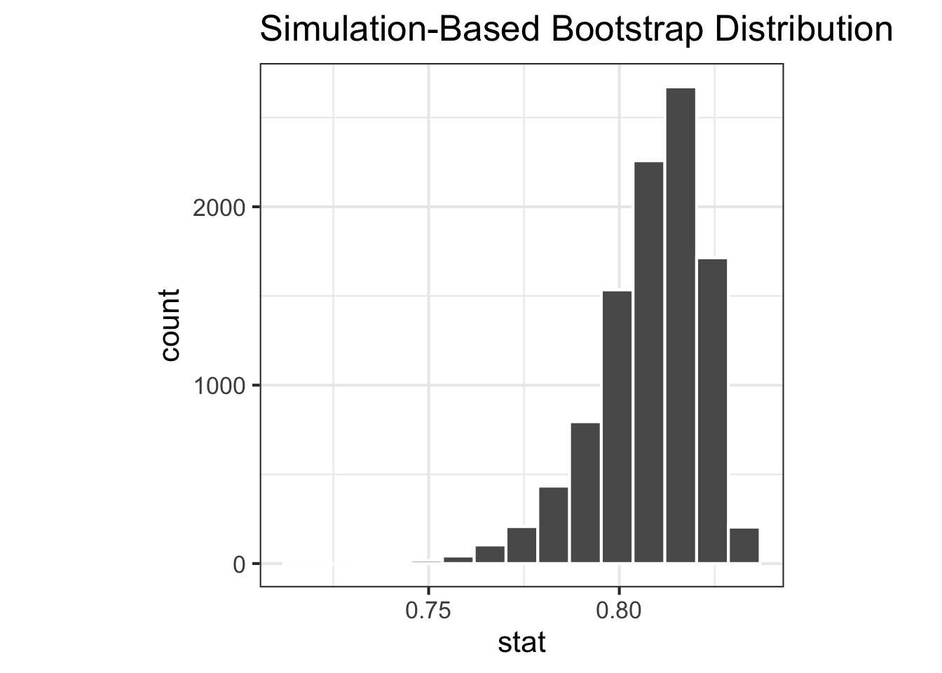
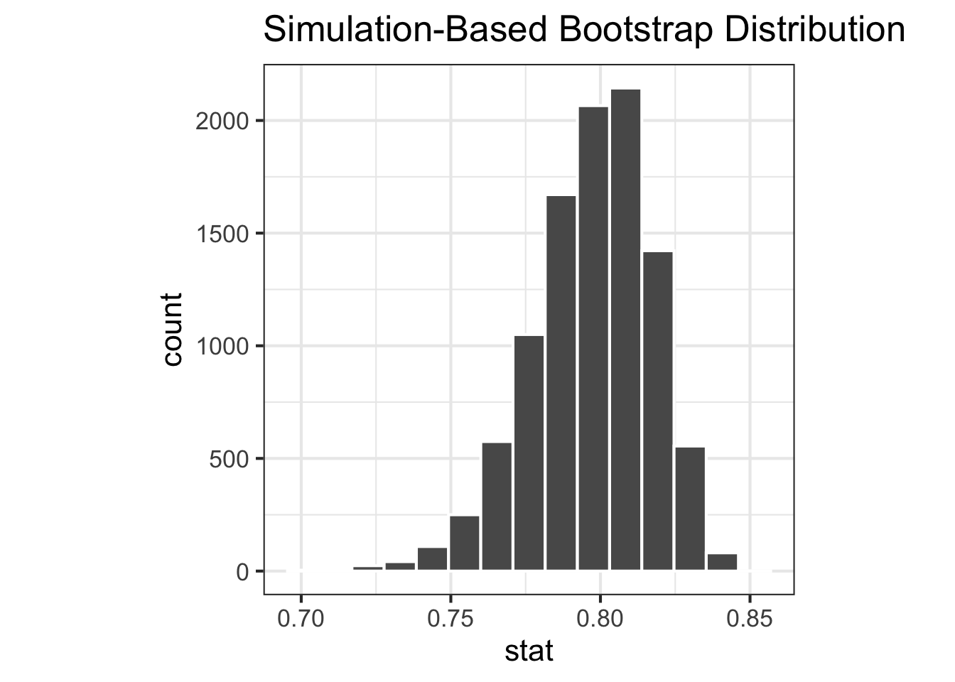
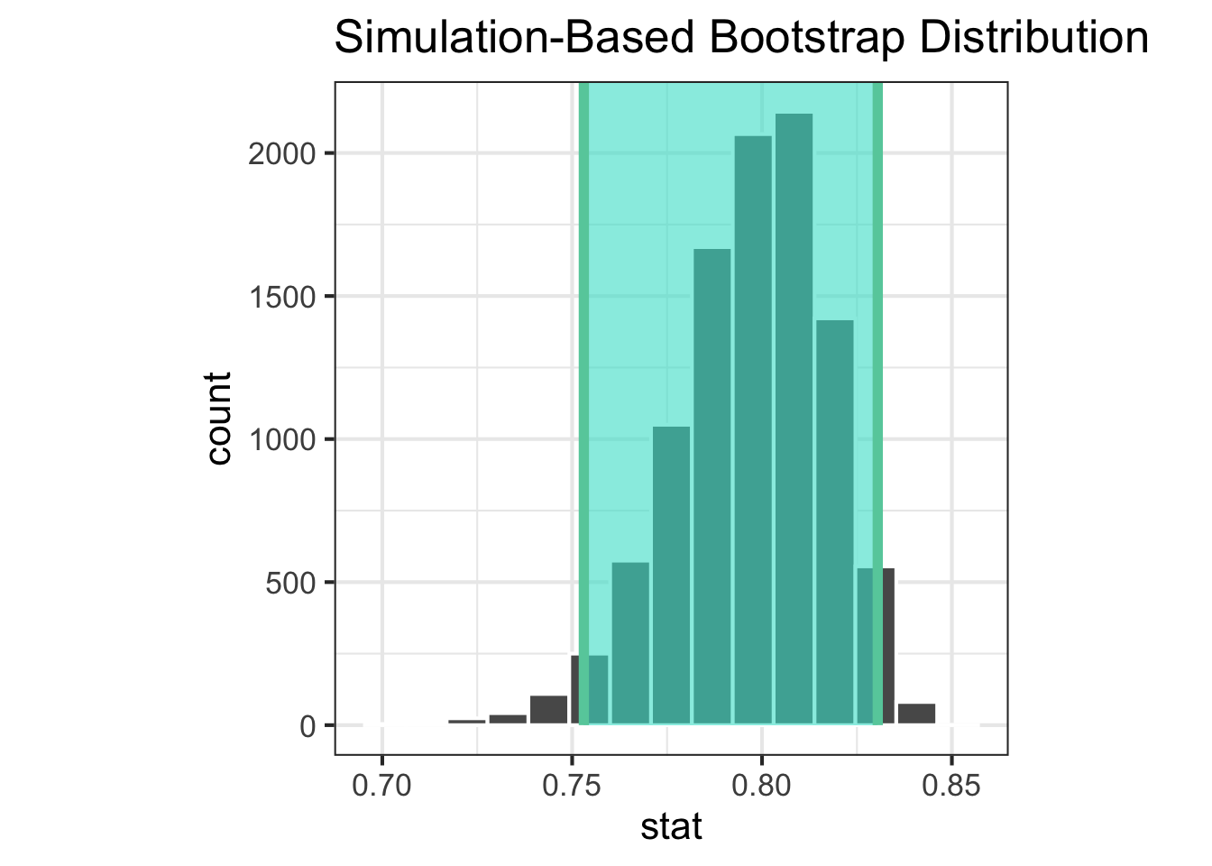
<- |> filter (environment == "env_a" ) |> specify (response = species) |> generate (reps = 10000 , type = "bootstrap" ) |> calculate (stat = stat_simpson)<- |> filter (environment == "env_b" ) |> specify (response = species) |> generate (reps = 10000 , type = "bootstrap" ) |> calculate (stat = stat_simpson)|> visualise ()|> visualise ()
Confidence interval
<- |> get_ci (level = 0.95 , type = "percentile" )<- |> get_ci (level = 0.95 , type = "percentile" )
# A tibble: 1 × 2
  lower_ci upper_ci
     <dbl>    <dbl>
1    0.774    0.828
# A tibble: 1 × 2
  lower_ci upper_ci
     <dbl>    <dbl>
1    0.753    0.830
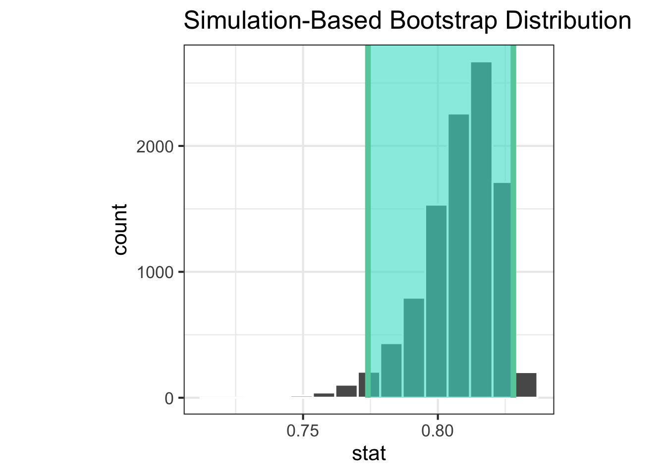
|> visualise () + shade_ci (endpoints = ci_simpson_a)|> visualise () + shade_ci (endpoints = ci_simpson_b)
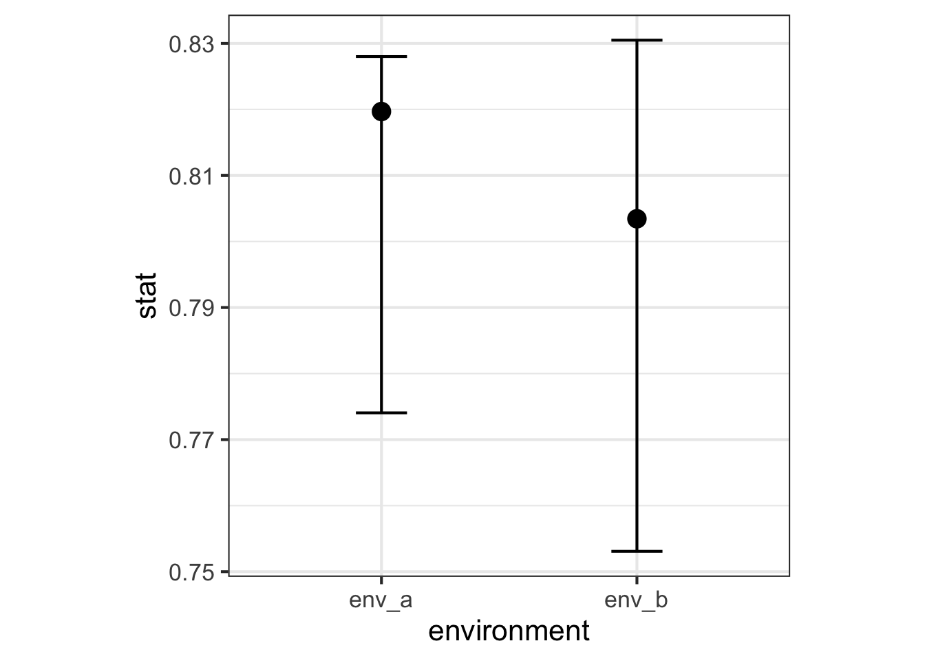
Plots
<- bind_rows (env_a = obs_simpson_a,env_b = obs_simpson_b,.id = "environment" <- bind_rows (env_a = ci_simpson_a,env_b = ci_simpson_b,.id = "environment" |> full_join (ci_simpson, by = join_by (environment)) |> ggplot (aes (x = environment, y = stat)) + geom_point (size = 4 ) + geom_errorbar (aes (ymin = lower_ci, ymax = upper_ci), width = 0.2 )