Introduction to R
Exercise 2
What is R?
R is a powerful, open-source programming language specifically designed for statistical computing, data analysis, and visualization.
How do I use R?
R can be used in a number of ways. In the next exercise session, we will install R on your computer, along with Rstudio, which is a friendly user interface for R. In this exercise, you will use R in your browser to explore its capabilities.
Note that once the webpage has loaded, you can edit the code in any of the boxes below (I strongly encourage you to do this!). Press the “Run code” button to run the code you have written. You will learn a lot through experimenting, and you can always reset the code box back to its original state with the “Start over” button.
Introduction to R
R as a calculator
R, like most programming languages, can perform arithmetic operations. It follows the order of operations used in mathematics. If you want to review that, you can do so in Chapter 1 of Duthie (2025).
You can use the following operators to write equations in R:
+: Addition-: Subtraction*: Multiplication/: Division^or**: Exponentiation%%: Modulus (remainder from division)%/%: Integer division
Use these to solve the questions below.
Programming concepts
While it is not required to be an experienced computer programmer to use R, there is still a set of basic programming concepts that new R users need to understand. We will cover these first. You do not need to memorise these things.
Objects
In R, data can be stored in objects. An object can be thought of as a container that holds data. You can create an object by assigning a value to a name using the assignment operator <-. In the example below, I assign the value 5 to the object x, and the value 10 to the object y. We can then perform maths or other operations using these objects.
x <- 5
y <- 10
x + yx <- 5
y <- 10
z <- 12
y / x * zObjects can hold any sort of data in R. It could be a single value like in the above example, multiple values, text, a whole dataset, or a plot.
Data types
In R, data can come in various types, and it’s important to understand these types to manipulate and analyse data effectively. Here are some of the most common data types in R:
- Numeric: Represents numbers and can be either integers or floating-point numbers. For example,
42and3.14are numeric values. - Character: Represents text or string data. Character values are enclosed in quotes, such as
"Hello, world!". - Logical: Represents boolean values, which can be either
TRUEorFALSE. - Factor: Used to represent categorical data. Factors are useful for storing data that has a fixed number of unique values, such as “Species A” and “Species B” for species ID.
Note that these are similar, but conceptually different, to the variables types we covered in the lecture. However, the variable types we covered are often encoded in R using these data types:
- Categorical variables:
- Nominal: we will generally use either a
characteror afactordata type. If used in a statistical test or to make a plot,characterdata is usually automatically converted to afactor. If your nominal variable is represented by a number (e.g., Forest1,2,3…), then it is usually best to explicitly convert it to either acharacteror afactor. - Ordinal: must be a
factor, as you can set the order of the levels witin the factor to the intended order. By default, the order will be determined by alpha-numeric order (A,B,C, 1,2,3).
- Nominal: we will generally use either a
- Quantitative variables
- Discrete:
numeric, and specifically, aninteger. R will infer the type of numeric data (integerordouble(with decimal)) from the data. - Continuous:
numeric, and specifically, adouble.
- Discrete:
Vectors
Vectors are one of the most basic data structures in R. A vector is a sequence of data elements of the same basic type. We will sometimes directly use vectors in this course, so it will be good to be familiar with them.
- Creating Vectors: You can create a vector using the
c()function, which stands for “combine” or “concatenate”. For example, here I create 3 vectors, and assign them to different objects:
Accessing Elements: You can access elements (position) of a vector using square brackets []. For example, to access the second element of character_vector:
Note that in R, the first position is [1], not [0] like in some programming languages.
Vector Operations: You can perform operations on vectors. These operations are applied element-wise. For example:
Note that every value in the vector gets multiplied and returned.
Vector Length: You can find the length (number of values in it) of a vector using the length() function:
Dataframes
Dataframes are like spreadsheets. They have rows and columns, and all columns are the same length. These are the primary way we will represent data in this course.
| species | mass_g | sex |
|---|---|---|
| blue_tit | 9.1 | male |
| blue_tit | 10.6 | male |
| sparrow | 27.3 | female |
We will come back to them soon.
Boolean and logical operators
Boolean operators are used to perform logical operations and return boolean values (TRUE or FALSE). We will use them in this course to describe our hypotheses. Here are the most common boolean operators in R:
- Comparison Operators: These operators compare two values and return a boolean value.
==: Equal to!=: Not equal to<: Less than>: Greater than<=: Less than or equal to>=: Greater than or equal to
For example, this bit of code should evaluate to TRUE:
And this should be FALSE:
100 == 100p <- 48
8 + p == 56q <- 24
r <- 88
1q + 65 > r- 1
- Any number > 64 will work.
We can now add in some logical operators:
- Logical Operators: These operators are used to combine multiple boolean expressions.
&: Logical AND|: Logical OR!: Logical NOT
For example, this bit of code should evaluate to TRUE, because both the first part 1 + 3 == 4 and the second part 5 >= 4 is TRUE:
Whereas this evaluates to FALSE, because only the first part is TRUE:
But if we change the & to an OR operator |, it evaluates to TRUE because at least one part of it is TRUE:
fruit_a <- "apple"
fruit_b <- "banana"

1(fruit_a != fruit_b) & (1.5 > 1.2)- 1
-
OR
|would also work here.
fruit_a <- "apple"
fruit_b <- "banana"

(fruit_a == fruit_a) | (35 + 12 > 47)
Functions
Functions perform tasks in R. Functions can take inputs, called arguments, and return outputs. We put the arguments inside the brackets. For example, in R there is a function called mean(). This function’s first argument x should be a vector of numeric data. The function then outputs the mean as a single numeric value. For example, here we assign a vector of tree heights (cm) to an object called trees. We then calculate the mean tree height using the mean() function.
Note that if we are going to supply arguments in the order that the function expects them, we do not have to tell the function which object is for each argument. Since mean() expects the first argument to be the vector you want the mean of, we can also write:
To find out what a function can do, and its arguments, use can write ?function_name, and the R helpfile will be returned for that function (e.g., ?mean). These helpfiles can be confusing at first, but the more you use R, the more they will make sense.
We will work with functions a lot in this course, so don’t worry if it still seems confusing.
Pipes
One of the final concepts I will introduce is the pipe operator |>. Note that you will often see it written as %>% when searching online. This is for historical reasons (R by default did not have a pipe operator until recently, so people had made their own). |> comes with R by default now, while %>% requires you to load a package called magrittr first (we will cover packages soon).
Pipes allow you to write code in a way that often makes more sense to people, especially non-programmers. To explain, here’s an example. Note that this is not real code, so you cannot run it.
Say I wanted to run 3 different functions on a dataframe called my_data. The functions are function_1(), function_2(), and function_3(). Imagine function_1() first transforms my data into the right scale, function_2() then performs a statistical test, and function_3() then makes a plot (again, these are not real functions, just for the example).
I could write that in a few ways. The first way would look like this:
- 1
-
The original data,
my_data, is passed tofunction_1(), and the result is stored inmy_data_1. - 2
-
The transformed data,
my_data_1, is then passed tofunction_2(), and the result is stored inmy_data_2. - 3
-
Finally, the data from
my_data_2is passed tofunction_3(), and the result is stored inmy_data_final.
While this method is quite clear to read, it creates a lot of objects that we might not want to do anything with. This is not a huge issue, but could become one if you are working with very large data sets.
We could also write it like this:
my_data_final <- function_3(function_2(function_1(my_data)))We can wrap functions within functions to put this whole operation on one line. This gets rid of those extra objects, having only a my_data_final as the output. However, the order in which the functions are written no longer matches the order in which they are run. In the above example, function_1() runs first, then function_2(), then function_3(). But they are written in reverse order when we read it left to right.
A final method of writing this makes use of pipes |>, and has the best of both approaches:
my_data_final <- my_data |> function_1() |> function_2() |> function_3()Pipes also allow us to spread our code over multiple lines, and the |> will look for the next bit of code on the next line if nothing comes after it:
my_data_final <-
my_data |>
function_1() |>
function_2() |>
function_3()All the above examples have the same my_data_final output, but are just written in different ways. The computer reads them all identically, so the main benefit is how readable your code is.
In this course, we will use pipes extensively, along with a set of packages that are designed for this kind of workflow.
1trees |> mean()- 1
-
Take the
treesvector, and then pipe|>it into themean()function.
The log() function performs a natural logarithm transformation of the data.
1trees |>
  log() |>
mean() - 1
-
Take the
treesvector, and then pipe|>it into thelog()function, then into themean()function.
Packages
An R package is a set of functions, data and/or information that someone else has written, that you can first load, then use in your own R code. Packages are written by other R users, and distributed for free via repositories, like The Comprehensive R Archive Network (CRAN).
R packages are often used to save you time. While all the functions in an R package are written with R, and you could write them again yourself, why bother? If someone else has done it already and shared it, fantastic! In this course, we are going to use two package “families”. They are tidyverse and tidymodels. Note that both start with tidy. Remember from the lecture, that tidy refers to a particular format of data, and these packages all assume your data will be in the format, and will always return data in that format. They are also all built with pipes in mind, and are designed to make complex programming tasks (especially those performed by data scientists, of which biology fits in well) very easy. We will cover these packages in detail soon, but know to use them you need to do two things:
- Install the package. This needs to be done once on your computer, using the
install.packages()command. For examples:
install.packages("ggplot2")This will install ggplot2, a package for plotting data. It will install it from CRAN by default, and probably (assuming you are in Sweden) will be downloaded from a server in Umeå.
- We now need to load the package, so that we can access it while we write code. To do that, we use the
library()function.
1library(ggplot2)- 1
-
Note that we no longer require the
"around the package name. But the function would still work if you did include them.
Below I have written some code that makes a plot using an inbuilt R dataset called iris using the package ggplot2. But if you try to run it, you will get an error. The ggplot2 package has already been installed, so fix the code by loading the ggplot2 package before the code that makes the plot.
1library(ggplot2)

iris |>
  ggplot(aes(x = Sepal.Length, y = Sepal.Width, colour = Species)) +
geom_point()- 1
-
Make sure to load the
ggplot2package before theggplot()function. Code is always executed top to bottom.
That was a lot of concepts in a very short amount of time! Take a break before the next section.
Running R locally
Follow the guide on how to install R and RStudio on your computer. Once they’re both installed, return to this section.
Welcome to RStudio
It should detect your R installation automatically, but if not, a window will open asking you to select it. If R does not appear here, I suggest you restart your computer first.
You should be met by a scene that looks like this:
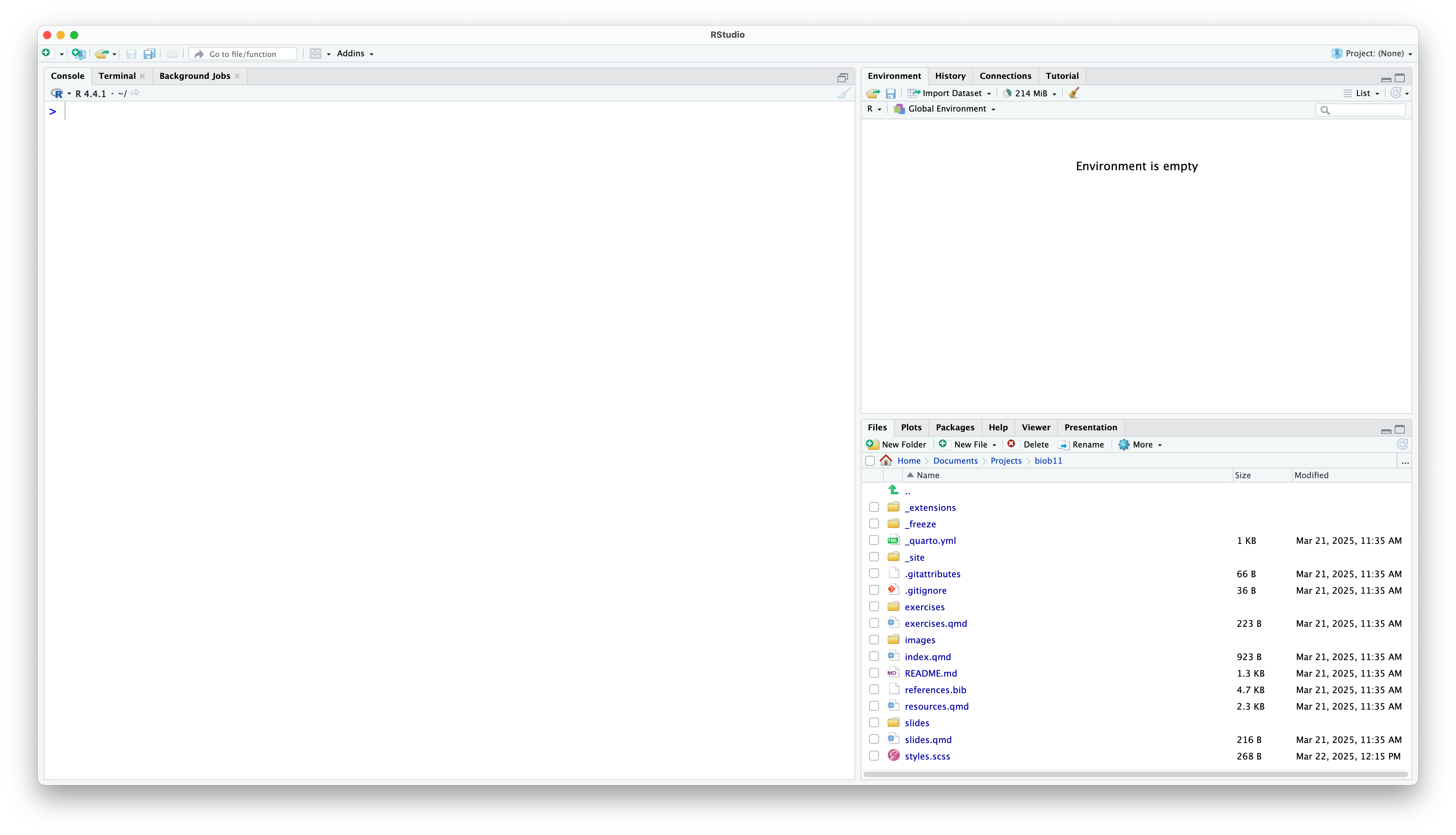
Rstudio is designed around a four panel layout. Currently you can see three of them. To reveal the fourth, go to File -> New file -> R markdown... This will open an RMarkdown document, which is a form of coding “notebook”, where you can mix text, images and code in the same document. We will use these sorts of documents extensively in this course. Give your document a title like “BIOB11 Exercise 4”. You can put your name for author, and leave the rest as default for now. Click OK. Now your window should look something like this:
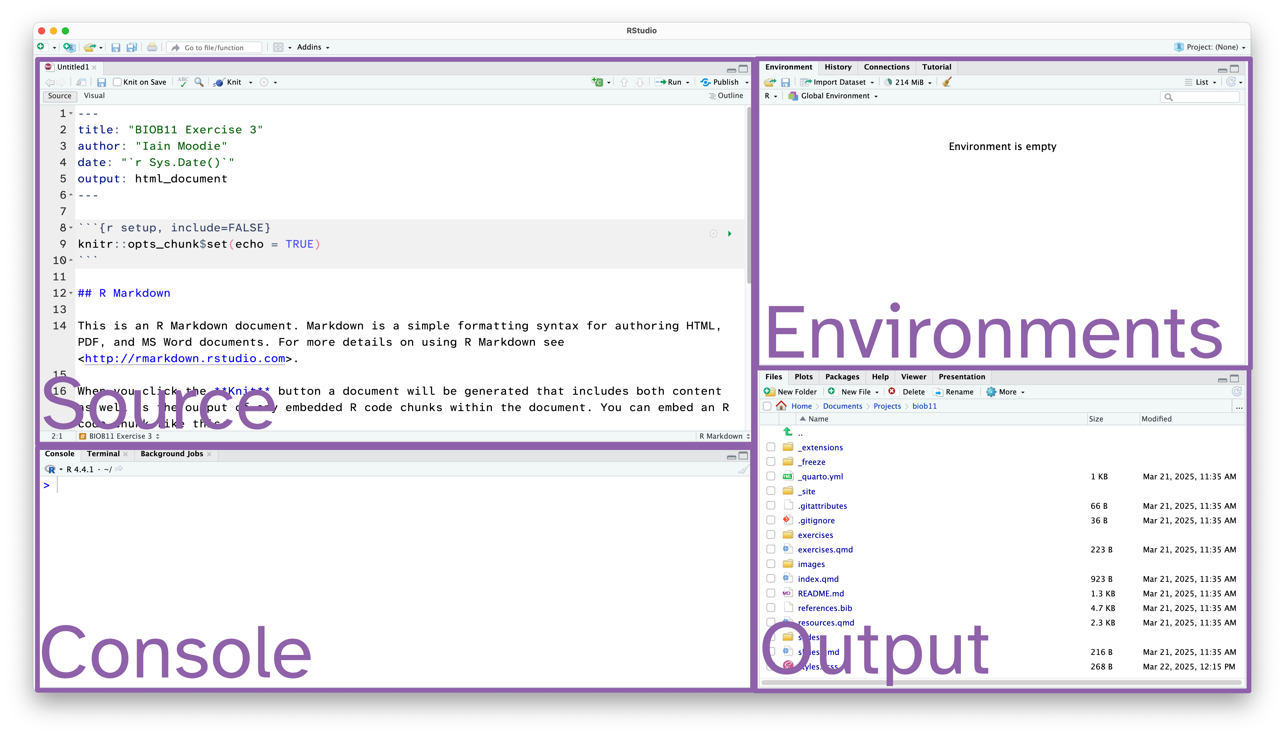
- Source: This is where we edit code related documents. Anything you want to be able to save should be written here.
- Console: the console is where R lives. This is where any command you write in the source pane and run will be sent to be executed.
- Environments: this panel shows you objects loaded into R. For example, if you were to assign a value to an object (e.g.
x <- 1), then it would appear here. - Output: this panel has many functions, but is commonly used to navigate files, show plots, show a rendered RMarkdown file or to read the R help documentation.
RMarkdown
RMarkdown is a file format for making dynamic documents with R. It combines plain text with embedded R code chunks that are run when the document is rendered, allowing you to include results and your R code directly in the document. This makes it a powerful tool for creating reproducible analyses, which are extremely important in science.
The RMarkdown document you opened has some example text and code. An RMarkdown document consists of three main parts:
YAML Header: This section, enclosed by
---at the beginning and end, contains metadata about the document, such as the title, author, date, and output format.Text: You can write plain text using Markdown syntax to format it. Markdown is a lightweight markup language with plain text formatting syntax, which is easy to read and write.
Code Chunks: These are sections of R code enclosed by triple backticks and
{r}. You can click the green arrow to run all the code in a code chunk, or run each line of code using the Run button, or by usingCtrl+Enter(Windows) or Cmd+Enter (macOS)When the document is rendered, the code is executed, and the results are included in the output.
Notice at the top left of the Source panel, there are two buttons: Source and Visual. These allow you to switch betwee two views of the RMarkdown document. The Source view is what you are looking at, and it is the raw text document. You can also use the Visual view, which allows you to work in a WYSIWYG (what you see is what you get) view, similar to Microsoft Office or other text editors. This “renders” your markdown code for you while you write. It also gives you a series of menus to help you format text, which means you do not need to learn how to write markdown code (although it is extremely simple, and you likely know some already).
Which ever view you prefer (and you can switch as often as you like), the code part stays the same. It is primarily there for editing the text around your code.
Important settings
Before we go any further, we need to change some default settings in RStudio.
While we are here, if you wanted to change the font size or theme, you can do that in the Appearance tab.
RStudio also has screenreader support. You can enable that in the Accessibility tab.
Working directory
I strongly recommend you create a folder where you save all the work you do as part of this course. I also recommend you make this folder in a part of your computer that is not being synced with a cloud service (iCloud, OneDrive, Google Drive, Dropbox, etc). These services can cause issues with RStudio. You can always backup your work at the end of a session.
Notice that now in your Output pane, in the files tab, you can see the contents of your folder (which is probably nothing currently). Let’s change that.
Saving your document
Let’s save this example RMarkdown document that RStudio has made for us. You do that exactly how you might expect.
The file should have appeared in your Output pane, with the extension .Rmd.
Installing R packages
In this course, we will use the tidyverse package, and the infer package. To install them you need to use the install.packages() function. Since we only need to do this once per computer, we should run this function directly in the Console panel.
install.packages("tidyverse")
install.packages("infer")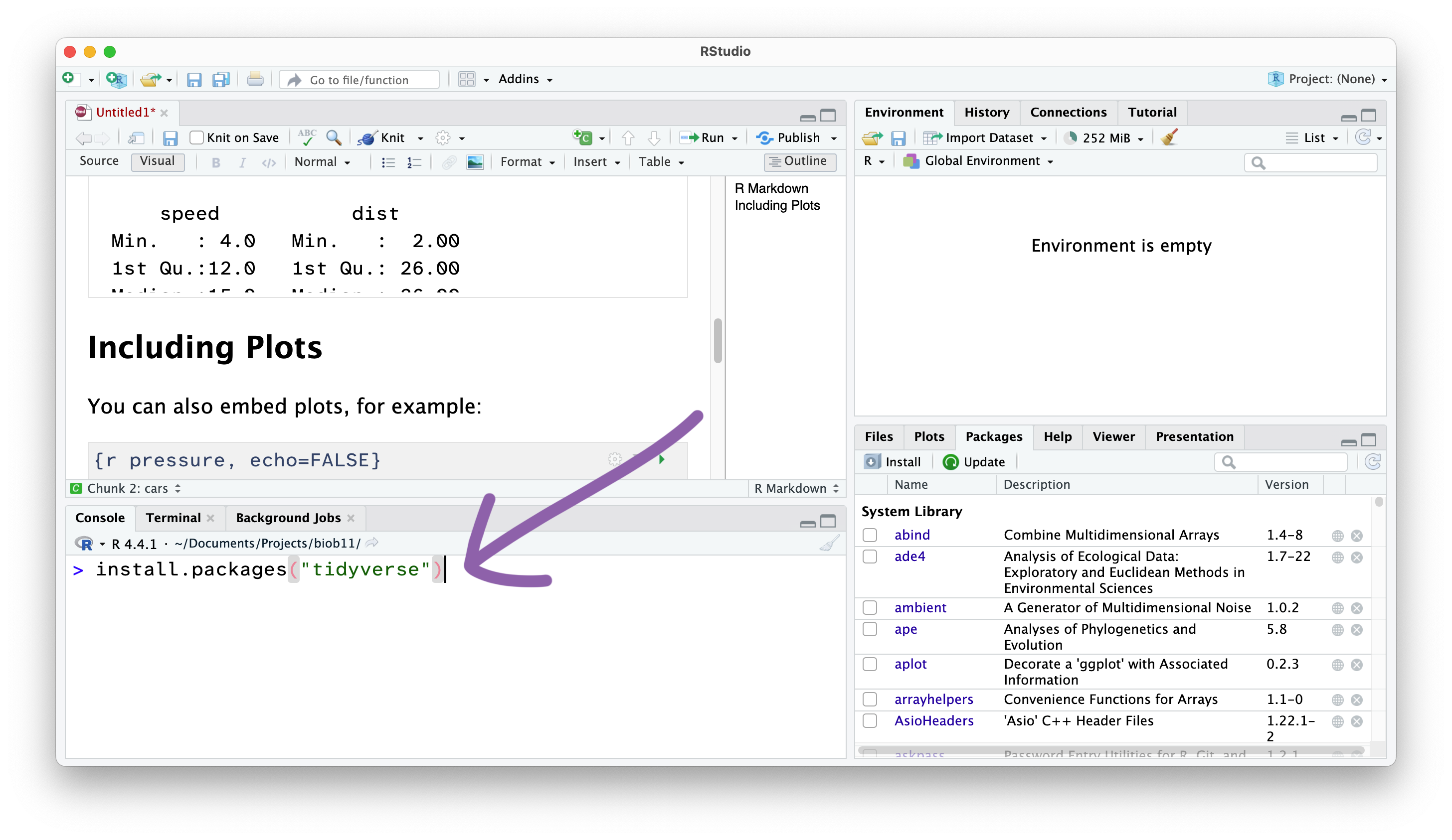
Let’s also install the package that contained the penguin data we used in the first exercise.
install.packages("palmerpenguins")From now on, we won’t write things directly in the Console, and instead write code in the RMarkdown document in the Source panel, which we then “Run” and send the Console.
Creating code cells
Code cells are where we write code in an RMarkdown document. This allows use to write normal text outside these sections.
NoteVisual view
To do that in the Visual view (where the text is rendered), go to Insert -> Executable Cell -> R.
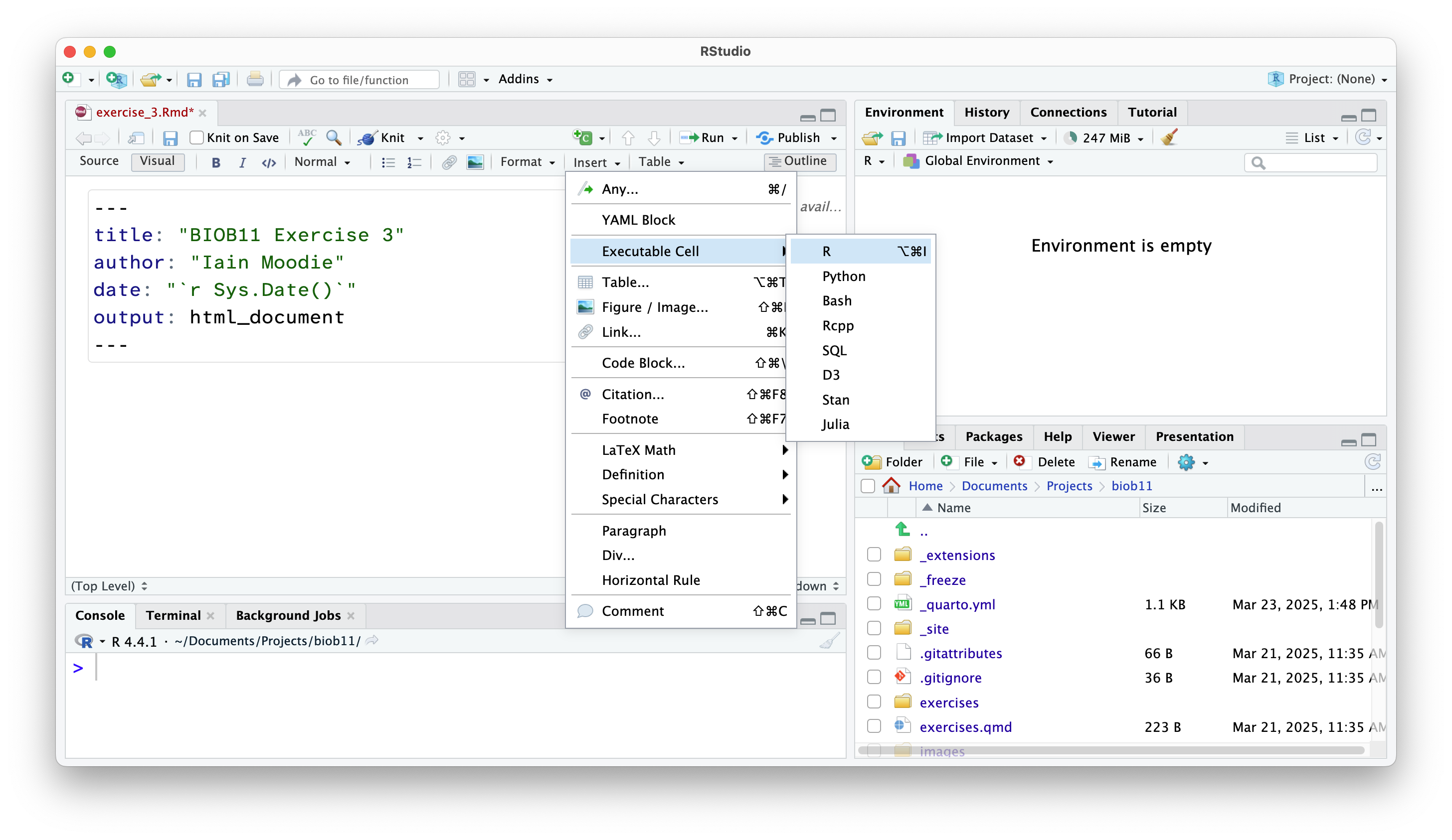
In both views, you can also use the shortcut Shift-Alt-I or Shift-Command-I.
Adding headings and text
Anywhere outside a code cell you can write normal text. In this course, you might find it helpful to write yourself notes alongside your code, so that you can come back to your notes during other exercises, the exam (open book), the group project, or later in your studies.
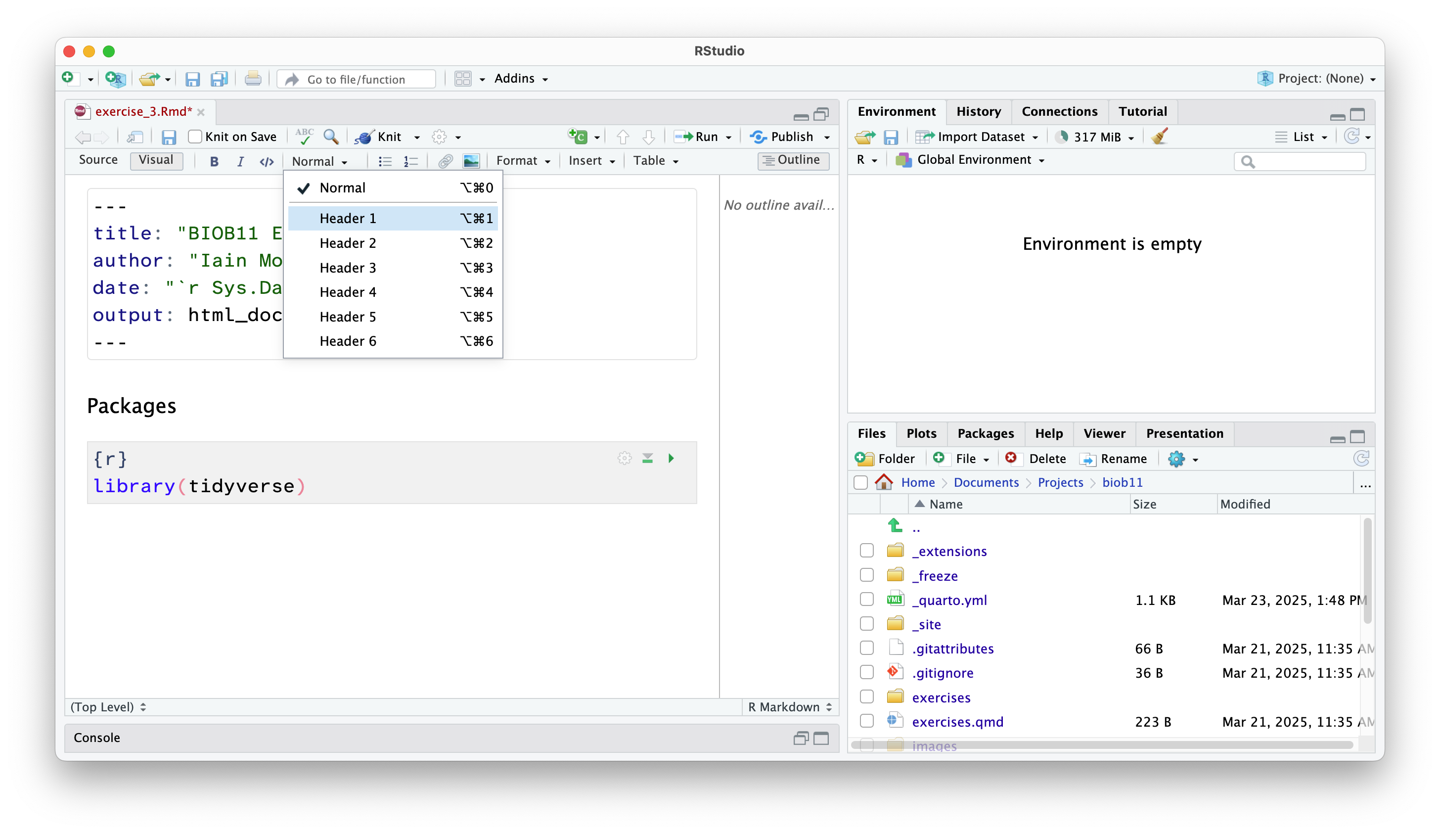
Along side normal text, you can structure an RMarkdown document using headings.
NoteVisual view
Change the type of text you are typing in the menu at the top:
Loading R packages
After installing an R package, we need to load it into our current R environment. We use the library() function to do that. Since we need this code to run every time we come back to this RMarkdown document, we should write it in the document. R code should always be executed “top to bottom”, so this bit of code should come right at the start.
library(tidyverse)
library(infer)
library(palmerpenguins)
If that worked, you will get a message that reads something similar to:
── Attaching core tidyverse packages ──────────────────────── tidyverse 2.0.0 ──
✔ dplyr     1.2.0     ✔ readr     2.2.0
✔ forcats   1.0.1     ✔ stringr   1.6.0
✔ ggplot2   4.0.2     ✔ tibble    3.3.1
✔ lubridate 1.9.5     ✔ tidyr     1.3.2
✔ purrr     1.2.1
── Conflicts ────────────────────────────────────────── tidyverse_conflicts() ──
✖ dplyr::filter() masks stats::filter()
✖ dplyr::lag()    masks stats::lag()
ℹ Use the conflicted package (<http://conflicted.r-lib.org/>) to force all conflicts to become errors

Attaching package: 'palmerpenguins'


The following objects are masked from 'package:datasets':

    penguins, penguins_raw
This message tells us which packages were loaded by the tidyverse package, and which functions from base R (the functions that come with R by default) have been overwritten by the tidyverse packages. Not all packages produce a message when they are loaded (for example, infer and palmerpenguins did not).