Regression modelling in R (and other things)

Exercise 6

Get RStudio setup

Each time you start a new exercise, you should:

1. Make a new folder in your course folder for the exercise (e.g. biob11/exercise_6)
2. Open RStudio
   • If you haven’t closed RStudio since the last exercise, I recommend you close it and then re-open it. If it asks if you want to save your R Session data, choose no.
3. Set your working directory by going to Session -> Set working directory -> Choose directory, then navigate to the folder you just made for this exercise.

Instructions

1. Create a new Rmarkdown document (File -> New file -> R markdown..). Give it a clear title. Delete any of the demo text not in the YAML frontmatter.
2. Download the dataset and move it into your working directory folder.
3. Load the tidyverse and infer packages.
4. Import the dataset using read_csv().
5. Use Headings so that your document is clear and easy to follow.
6. Write your answers to the questions as text in the document.

What approach to use?

You need to decide whether to use a hypothesis test or a confidence interval. During the exercise, you should use both approaches at some point.

Note🤔 If you use a hypothesis test

1. Produce a figure using ggplot() using the data that reflects the research question.
2. State a null and alternative hypotheses.
3. State the sample statistic you will calculate, and why this addresses the research question.
4. Explain how you will derive a null distribution, and why this is valid for the research question.
5. Calculate the test statistic, and compare it with the null distribution to calculate a p-value.
6. Write a conclusion statement that directly addresses the research questions, and references key results from your analysis.

Note🎯 If you use a confidence interval

1. Produce a figure using ggplot() using the data that reflects the research question.
2. State the sample statistic you will calculate, and why this addresses the research question.
3. Explain how you will derive a sampling distribution and how you will calculate a confidence interval from it, and why this is a valid approach.
4. Calculate the test statistic.
5. Derive a sampling distribution, and use it to calculate a confidence interval.
6. Write a conclusion statement that directly addresses the research questions, and references key results from your analysis.

You will need to use past exercies, slides, the course book and the infer webpage for help with implementing your ideas. Try to use them first before asking for help. But if you’re stuck, then please ask!

Öland Orchids

Illustration of the two study species, the orchids Gymnadenia conopsea (a) and Gymnadenia densiflora (b) that differ in plant height and floral display and particularly in flowering time (c), as shown at a site where they co-occur: G. conopsea (left) has initiated fruit development while G. densiflora (right) is still in bud (Chapurlat et al. 2020).

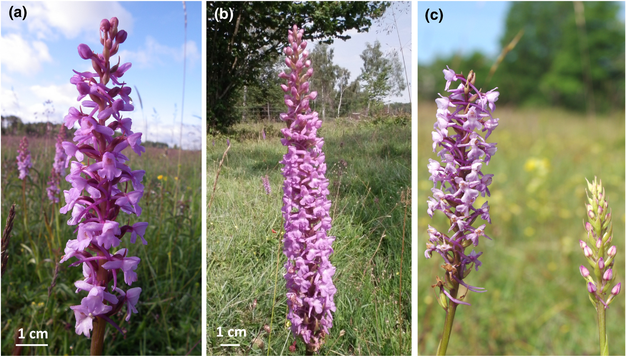
Gymnadenia conopsea and Gymnadenia densiflora are two closely related perennial orchids that differ in key floral traits affecting pollination and in their primary pollinator species. This dataset was collected from 10 populations on Öland by Chapurlat et al. (2020). For more information, have a look at the paper.

The dataset can be downloaded as a csv file from GitHub.

The variables are as follows:

• species: species name (Gymnadenia conopsea or Gymnadenia densiflora)
• population: population identifier where the plant was sampled
• plant_height_cm: plant height in centimetres
• corolla_area_mm2: corolla (flower) area in square millimetres
• spur_length_mm: spur length in millimetres
• first_flower_day: day of year (Julian day) when the first flower was observed (1 = 1st Jan)
• flowers: number of flowers on the plant
• fruits: number of fruits produced on the plant
• mean_fruit_mass_mg: mass per fruit (mean of three fruits) in milligrams

Floral correlations

The researcher’s want to know if there are correlations between key phenotypic traits. Correlations between traits can generate indirect selection: selection on one trait may cause a correlated response in another, even if that other trait is not under direct selection.

Note✅ Task

1. Within each species, do taller plants tend to have more flowers?
2. Is the relationship strong or weak?
3. Does it differ between species?

Note✅ Task

1. Within each species, do plants with longer spurs tend to have larger corolla areas?
2. Is the relationship strong or weak?
3. Does it differ between species?

Note✅ Task

1. Describe the differences in number of fruits and fruit mass between the species? Which species produces fewer, but heavier fruits, and which one produces many, but lighter fruits?
2. Are the differences “real”, or could they be due to chance?

Selection gradients

A selection gradient quantifies the relationship between a trait and fitness, measuring the strength and direction of natural selection acting on that trait. Fitness is an individual’s contribution to the next generation, typically measured as reproductive success. Directional (linear) selection can be captured well using the slope of a linear regression.

While the authors did not quantify fitness directly, they did measure two traits that once combined provide a good estimate of a plant’s reproductive success. Fruit mass is likely a product of the number of seeds within a fruit, so mean_fruit_mass_mg \(\times\) fruits will give us a variable that is a proxy for number of seeds, which is a good estimate of an individual’s fitness.

Note✅ Task

Make a new variable in the dataset called fitness using mutate()

data <-
  data |>
  mutate(fitness = ______ * ______)

1. Within the G. conopsea "kvinneby" population, describe the direction and strength of selection on spur_length_mm. Describe the results of your regression verbally, for example:

“For every mm increase in spur length, an individual is expected to have ______ mass of fruits.”

2. Given this relationship, how might you expect the population to change in the future?

3. What fitness does your model predict for a spur_length_mm of 15 mm?

Note✅ Task

To compare selection gradients between populations or species, we need to standardise them first.

First, we need to transform fitness to relative fitness. To do that, we could divide an individual’s fitness by the mean fitness of the population. Since we also have two species that are both present at some populations, we should make sure to group by species as well.

data <-
  data |>
  drop_na(fitness) |>
  group_by(species, population) |>
  mutate(relative_fitness = fitness / mean(fitness)) |>
  ungroup()

Next, we need to standardise any traits we wish to study. One way to do that is to mean standardise them, like we did for fitness.

data <-
  data |>
1  drop_na(______) |>
  group_by(species, population) |>
  mutate(relatve______ = ______ / mean(______)) |>
  ungroup()

1

Replace ______ with you variable name you are interested in.

Now, using standardised data, fit a linear regression model that allows you to compare the relative strength of selection on first_flower_day between the two species in the Graborg population¹.

1. Describe the relative strengths and directions of selection. Highlight differences between the species.

Logistic predictions

Suppose we want to build a model to help amateur naturalists identify which of the two species they are looking at.

Note✅ Task

1. By plotting your data, identify two variables you think help differentiate these species the best (you cannot use population).
2. Use your chosen variables as explanatory variables in a logistic regression model, with species as the response variable.
3. Which of your variables is helping to predict the species the most? Why?

Submit your work

Note✅ Final task

Once you’re done, knit your document to a HTML file.

it will have been saved next to wherever your .Rmd file is saved.

Upload your .html file as your assignment for this exercise in Canvas.

References

Chapurlat, E., I. Le Roncé, J. Ågren, and N. Sletvold. 2020. Divergent selection on flowering phenology but not on floral morphology between two closely related orchids. Ecology and Evolution 10:5737–5747.

Footnotes

1. note that this has been coded as two different populations in the dataset, one for each species. Look at the data to see what they’re called