Make a new folder in your course folder for the exercise (e.g. biob11/exercise_7)
Open RStudio
If you haven’t closed RStudio since the last exercise, I recommend you do so and then re-open it. If it asks if you want to save your R Session data, choose no.
Set your working directory by going to Session -> Set working directory -> Choose directory, then navigate to the folder you just made for this exercise.
Create a new Rmarkdown document (File -> New file -> R markdown..). Give it a clear title.
Please ensure you have followed the step above before you start!
Effect of fertilizer application on crop growth
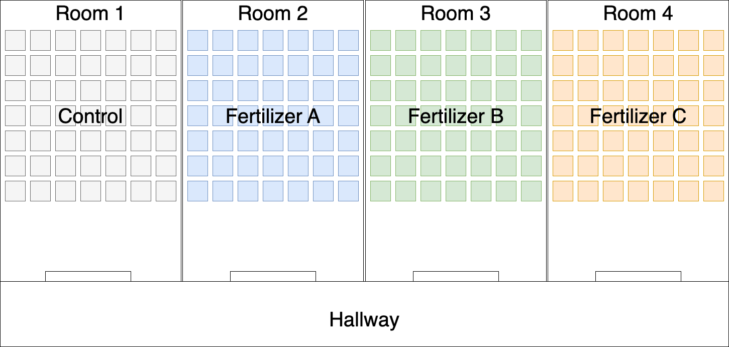
Some researchers at Lund University want to understand the effectiveness of three fertilizers on promoting crop growth. To do that, they construct 7 x 7 experimental arrays of plant pots for each treatment (Figure 1). Each experimental array is kept in a seperate green house chamber (room). The control pots were filled with a standardised soil mixture. The treatment plots were filled with the same standardised soil mixture plus the addition of the fertilizer. Already germinated seedlings were randomly assigned to pots and planted. Plants were kept in the greenhouses, and watered regularly.
Figure 1: The layout of the experiment in the greenhouse chambers.
After 30 days, the researchers used a knife to cut all of the plant’s biomass that was above ground. Using an oven, they dried each plant for 24 hours before recording the mass in grams using a balance.
The results of the experiment are stored in a csv file here: Link to data
Analysis
While working on your analysis, answer the questions below:
General
What (statistical) population are the researchers trying to make inferences about?
Data handling and plotting
Load the tidyverse and infer packages.
Import the dataset using read_csv().
What sort of variables are dry_mass_g and treatment?
Check the data for mistakes.
Make an illustrative plot of the dataset.
Descriptive statistics
Report the following statistics:
The overall mean of dry_mass_g.
The mean of dry_mass_g for each treatment group.
The standard deviation of dry_mass_g for each treatment group.
Is there a difference in means between the groups?
This sort of analysis is called an ANOVA (ANalysis Of VAriance). Specifically, it is a one-way ANOVA, as we are interested in the effect of one categorical variable on a continuous variable.
Specify which is your response and explanatory variable.
3
Calculate the observed statistic.
4
Print the observe statistic to the console.
To generate a null distribution, we can use a permutation approach, where we shuffle the assigned categories and calculate our statistic many many times. Generate a null distribution.
Pipe your null_dist object into visualise(). You can change the number of bins if you wish.
2
Plot your observed_stat, and specify that the direction should be greater. Our statistic is a ratio, so is naturally bounded at 0.
3
You can change the axis labels to make the plot more clear.
Use your observed statistic and your null distribution to calculate a p-value.
Code hint
null_dist |>get_p_value(obs_stat = observed_stat, direction ="greater")
What are your conclusions? State them both clearly in terms of the null hypothesis and as if you were describing them to someone who does not know about statistics.
Post-hoc analysis
You might suspect that one particular treatment group is causing your ANOVA result. As the ANOVA does not let you say which group(s) are different from the global mean, there is often the need for a post-hoc (Latin for “after this”) analysis.
A post-hoc analysis are tests you do after you have seen your data (and often some results). It is important to differentiate this analysis from your original one, as you did not plan to do it and (remember from the slides) the more tests you do, the more likely you are to find a low p-value by chance alone. As such unethical researchers may be tempted to propose additional tests as if they were part of the original plan (HARKing) and to keep doing analyses until they find a low p-value (p-hacking or data-dredging). Both of these practises have likely contributed to the replication crisis in many field, including biology.
In this case, we will perform a post-hoc analysis of the difference of means between one of the treatments and the control. We want to know if it has had a statistically significant effect on the growth of the crops.
Filter the dataset
Use filter to produce another dataset that only has the treatment groups you are interested in.
Specify which is your response and explanatory variable.
3
Calculate the observed statistic, specifiying the order as treatment - control. That way a positive number indicates that the treatment made the crops grow bigger.
Specify which is your response and explanatory variable.
3
Our hypothesis is that our response variable is independant of our explanatory variable.
4
What simulation approach should you use here?
5
From each of our simulated samples, calculate the test statistic.
Plot the null distribution and the observed statistic.
Code hint
null_dist |>1visualise(bins =15) +2shade_p_value(obs_stat = observed_stat, direction ="_____") +3labs(x ="______")
1
Pipe your null_dist object into visualise(). You can change the number of bins if you wish.
2
Plot your observed_stat, and specify that the direction of the hypothesis?
3
You can change the axis labels to make the plot more clear.
Use your observed statistic and your null distribution to calculate a p-value.
Code hint
null_dist |>get_p_value(obs_stat = observed_stat, direction ="______")
What are your conclusions of the post-hoc analysis?
Correcting p-values for multiple testing
If you had gone on to perform more post-hoc tests (like testing other treatments against the control), you might want to perform a correction to your p-values that recognises that the more tests you do, the more likely you are to find a low p-value by chance.
One way to do this is the Bonferroni correction. This simply devides your \(\alpha\) value (the p-value at which you deem a test to be significant) by the number of tests you did. So if we compared each fertilizer to the control (3 comparisons, 3 tests) we should use an \(\alpha\) value of \(\frac{0.05}{3}=0.0166\) (assuming our prior \(\alpha=0.05\)). You can achieve the same result by keeping \(\alpha=0.05\) and multiplying all your p-values by the number of tests you performed.
Experimental design
Read again the description of the experiment and look at Figure 1.
Identify one aspect of their experimental design which will have helped them collect unbiased data.
Suggest one way in which the researchers could improve their experimental design?