Make a new folder in your course folder for the exercise (e.g. bioc13/exercise_2)
Open RStudio
If you haven’t closed RStudio since the last exercise, I recommend you close it and then re-open it. If it asks if you want to save your R Session data, choose no.
Set your working directory by going to Session -> Set working directory -> Choose directory, then navigate to the folder you just made for this exercise.
Create a new Rmarkdown document (File -> New file -> R markdown..). Give it a clear title.
Please ensure you have followed the step above before you start!
Loading R packages
If you installed the R packages from the last session, you do not need to reinstall them, only load them into our current R environment. We use the library() function to do that. Since we need this code to run every time we come back to this RMarkdown document, we should write it in the document. R code should always be executed “top to bottom”, so this bit of code should come right at the start.
Note✅ Task
Make a code cell and use the library() function to load the tidyverse and infer packages:
library(tidyverse)library(infer)
You are now ready for today’s exercise!
Effect of fertilizer application on crop growth
An image of a greenhouse.
Researchers at Lund University want to understand the effectiveness of three fertilizers on promoting crop growth. To do that, they construct experimental arrays of plant pots. The control pots were filled with a standardised soil mixture. The treatment plots were filled with the same standardised soil mixture plus the addition of the fertilizer. Already germinated seedlings were randomly assigned to pots and planted. Plants were kept in the greenhouses, and watered regularly.
After 30 days, the researchers used a knife to cut all of the plant’s biomass that was above ground. Using an oven, they dried each plant for 24 hours before recording the mass in grams using a balance.
The results of the experiment are stored in a .csv file on GitHub or Canvas.
Note✅ Task
Download the dataset.
Once downloaded, you should move it to your working directory folder for this exercise before continuing.
Import the data
We will now import the crop_growth.csv dataset.
Note✅ Task
Make another code cell. Load the crop_growth.csv data file using the read_csv() function and assign it to an object named crop_data.
crop_data <-read_csv("crop_growth.csv")
Explore the data
Note✅ Task
In your RMarkdown document, using text below the code cell, answer the following questions:
How many rows of data are in the dataset?
What is the unit of observation in this dataset? In other words, what does each row represent?
What sort of variables are in the dataset (continuous, discrete, nominal, ordinal)?
What is the minimum and maximum dry_mass_g the researchers recorded?
Plot the data
Below I have provided you with the base ggplot() function, but you need to add a geom_ to it.
crop_data |>1ggplot(aes(x = treatment, y = dry_mass_g))
1
To add some geometry add a + to the end of this line, then copy the geom_ onto the next line
Some examples geometries could be:
geom_boxplot()
geom_violin()
geom_jitter(width =0.1)
Note✅ Task
Try each of the geom_s out, and decide which you think is best. You can also add more than one geom_ to a plot, just add a + at the end of a line, then put the second geom_ on the next line.
Calculating the observed statistic
Our research question is:
Is there a difference in mean dry_mass_g between treatment groups?
Since we have more than two groups, this sort of analysis is called an ANOVA (ANalysis Of VAriance). Specifically, it is a one-way ANOVA, as we are interested in the effect of one categorical variable (with >2 groups) on a continuous variable.
Note✅ Task
In your RMarkdown document, using text below the code cell, answer the following questions:
State the null and alternative hypothesis.
What is the test statistic we use in an ANOVA?
In a new code cell, calculate the observed test statistic
Specify which is your response and explanatory variable.
3
Calculate the observed statistic. To see the possible names you can use, write ?calculate to open the help files for that function.
4
Print the observe statistic to the console.
Confidence interval approach
Since the statistic used in an ANOVA unitless ratio (always greater than 0), a confidence interval is not a very helpful in this case.
If you wanted to use a confidence interval for this question, you could calculate a confidence interval for the mean of each group, and then compare them.
If you want to do that, some code is below, but feel free to move onto the hypothesis test, which is more useful here.
NoteConfidence interval around the mean of each group
First split the treatments into their own datasets with filter():
Since our null hypothesis is that there is no relationship between two variables (i.e., dry_mass_g and treatment are independent), we can use permuation (shuffling one of the columns) to simulate a null distribution.
Note✅ Task
In a new code cell, generate a null distribution using the code below:
The name of the dataset (I called mine crop_data).
2
Specify which is your response and explanatory variable.
3
Our hypothesis is that our response variable is independant of our explanatory variable.
4
Simulate data using permuations. This may take a few seconds depending on your computer.
5
From each of our simulated permutation samples, calculate the test statistic.
Compare your observed against the null
In order to see if our statistic could have been observed due to chance, we should now compare the observed statistic to the null distribution.
Note✅ Task
In a new code cell, plot the null distribution and the observed statistic using the code below:
null_dist_f |>1visualise() +2shade_p_value(obs_stat = obs_f, direction ="greater") +3labs(x ="______ statistic")
1
Pipe your null_dist object into visualise().
2
Plot your observed_stat, and specify that the direction should be "greater". Our statistic is naturally bounded at 0, so we are not interested in the left side of the distribution.
3
You can change the axis labels to make the plot more clear.
Calculate a p-value
Let’s count up the number of simulations in our null distribution that produced statistics as or more extreme than our observed statistic, to get a p-value.
Note✅ Task
In a new code cell, use your null distribution to calculate a p-value:
null_dist_f |>get_p_value(obs_stat = obs_f, direction ="greater")
Did the fertilizers affect the growth of the crops?
Note✅ Task
In your RMarkdown document, using text below the last code cell, answer the following question:
What are your conclusions? State them both clearly in terms of the research question and null hypothesis. How would you describe them to someone who does not know much about statistics? Make reference to your p-value and your figure.
Save your work! Take a break! Then move on to the next question when you’re ready.
Species co-occurences in benthic communities
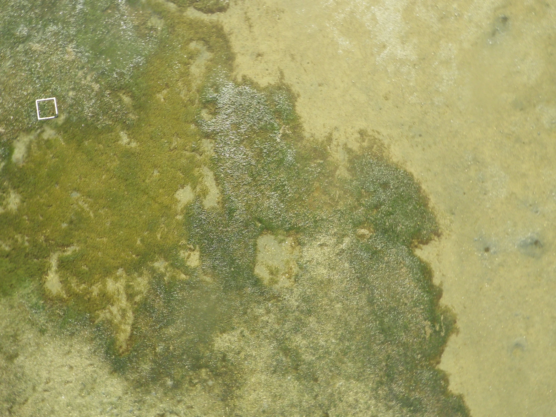
An illustration of the visual contrast between seagrass meadows (left hand side) and bare sediment sandflats (right hand side). Picture taken by Roman Zajac at Kaipara harbour, New Zealand. The white rectangle encompasses 0.5 × 0.5 m
Co-occurrence patterns of species across a landscape may arise due to shared habitat preferences, dispersal patterns, community interactions (e.g. facilitation, competition) or the interaction of these processes. To understand if communities differ in species composition and/or abundance between open sand and sea grass habitats in a shallow bay, researchers conducted snorkling transects and recorded the number of 6 important benthic species.
The dataset the researchers collected can be found as a .csv file on GitHub or on Canvas.
Note✅ Task
Download the dataset.
Once downloaded, you should move it to your working directory folder for this exercise before continuing.
Import the data
We will now import the benthic_species.csv dataset.
Note✅ Task
Make another code cell. Load the benthic_species.csv data file using the read_csv() function and assign it to an object named benthic_data.
benthic_data <-read_csv("benthic_species.csv")
Explore the data
Note✅ Task
In your RMarkdown document, using text below the code cell, answer the following questions:
How many rows of data are in the dataset?
What is the unit of observation in this dataset? In other words, what does each row represent?
What sort of variables are in the dataset (continuous, discrete, nominal, ordinal)?
Plot the data
Here’s some code to help you make a bar plot, which is a nice way to display categorical data:
benthic_data |>1ggplot(aes(x = ______, fill = ______)) +geom_bar()
1
This will display one of the variables on the x axis, and the other by filling the bar with colour
Note✅ Task
Use the code above to make a plot. Try swapping which variable is mapped to x and which is mapped to fill. Which do you think is clearer?
Calculating the observed statistic
The researchers want to know if the community compositions of the habitats are the same or different. In other words, are some species more likely to be found in one habitat than the another, or are they randomly spread across the bay.
To do that, we will use a \(\chi^2\) statistic. Recall that a \(\chi^2\) statistic measures how different an observed distribution is from an expected distribution. In this case, how different the observed distribution of species is in each habitat from the “null” expected distribution of equally split between habitats (each species is found 50% of the time in each of the two habitats).
Note✅ Task
In your RMarkdown document, using text below the code cell, answer the following questions:
State the null and alternative hypothesis.
In a new code cell, calculate the observed \(\chi^2\) test statistic. Since the \(\chi^2\) statistic itself includes a null hypothesis (as in we need to supply the expected value), we need to use hypothesise() here when calculating it:
Specify which is your response and explanatory variable.
3
Calculate the observed statistic. To see the possible names you can use, write ?calculate to open the help files for that function.
4
Print the observe statistic to the console.
Confidence interval approach
Like the \(F\) statistic in an ANOVA, \(\chi^2\) is unitless ratio (always greater than 0), so a confidence interval is not a very helpful in this case.
Null hypothesis testing approach
A general approach to hypothesis testing
Generating a null distribution
Since our null hypothesis is that there is no relationship between two variables (i.e., species and habitat are independent), we could use permuation (shuffling one of the columns) to simulate a null distribution.
Note✅ Task
In a new code cell, generate a null distribution using the code below:
Specify which is your response and explanatory variable. In this case, it doesn’t matter for the statistic, but you might have a preference depending on what you think is causing the relationship.
3
Our hypothesis is that our response variable is independant of our explanatory variable.
4
Simulate data using permuations. This may take a few seconds depending on your computer.
5
From each of our simulated permutation samples, calculate the test statistic.
Compare your observed against the null
In order to see if our statistic could have been observed due to chance, we should now compare the observed statistic to the null distribution.
Note✅ Task
In a new code cell, plot the null distribution and the observed statistic using the code below:
null_dist_chi2 |>1visualise() +2shade_p_value(obs_stat = obs_chi2, direction ="greater") +3labs(x ="______ statistic")
1
Pipe your null_dist object into visualise().
2
Plot your observed_stat, and specify that the direction should be "greater". Our statistic is naturally bounded at 0, so we are not interested in the left side of the distribution.
3
You can change the axis labels to make the plot more clear.
Calculate a p-value
Let’s count up the number of simulations in our null distribution that produced statistics as or more extreme than our observed statistic, to get a p-value.
Note✅ Task
In a new code cell, use your null distribution to calculate a p-value:
null_dist_chi2 |>get_p_value(obs_stat = obs_chi2, direction ="greater")
Are the community compositions of the habitats different?
Note✅ Task
In your RMarkdown document, using text below the last code cell, answer the following question:
What are your conclusions? State them both clearly in terms of the research question and null hypothesis. How would you describe them to someone who does not know much about statistics? Make reference to your p-value and your figure.
Save your work! Take a break! Then move on to the next question when you’re ready.
Bergmann’s rule
The Atlantic marsh fiddler crab, Minuca pugnax, lives in salt marshes throughout the eastern coast of the United States. Historically, M. pugnax were distributed from northern Florida to Cape Cod, Massachusetts, but like other species have expanded their range northward due to ocean warming.
The pie_crab.csv dataset is from a study by Johnson and colleagues at the Plum Island Ecosystem Long Term Ecological Research site.
13 marshes were sampled on the Atlantic coast of the United States in summer 2016
Spanning > 12 degrees of latitude, from northeast Florida to northeast Massachusetts
Between 25 and 37 adult male fiddler crabs were collected, and their carapace size (mm) recorded
The dataset was collected to test Bergmann’s rule:
One of the best-known patterns in biogeography is Bergmann’s rule. It predicts that organisms at higher latitudes are larger than ones at lower latitudes. Many organisms follow Bergmann’s rule, including insects, birds, snakes, marine invertebrates, and terrestrial and marine mammals (Johnson et al. 2019).
Note✅ Task
Download the dataset.
Once downloaded, you should move it to your working directory folder for this exercise before continuing.
Import the data
We will now import the pie_crab.csv dataset.
Note✅ Task
Make another code cell. Load the pie_crab.csv data file using the read_csv() function and assign it to an object named pie_crab.
pie_crab <-read_csv("pie_crab.csv")
Explore the data
Note✅ Task
In your RMarkdown document, using text below the code cell, answer the following questions:
How many rows of data are in the dataset?
What is the unit of observation in this dataset? In other words, what does each row represent?
What populations (statistical use of the word) could we make inferences about using this data?
Plot the data
Note✅ Task
Try and figure out how you would use ggplot() and geom_point() to plot latitude on the x axis and size on the y axis.
Copy some code you used in previous questions and edit it.
Calculating the observed statistic
The research question is:
Does Minuca pugnax follow Bergmann’s rule?
Note✅ Task
In your RMarkdown document, using text below the code cell, answer the following questions:
Use the slides to help you decide what statistic would help you answer this question. What test statistic will you use? Why?
In a new code cell, calculate the observed test statistic:
This question could also be answered using a hypothesis test, but we’ve already done enough of these. Try to use the confidence interval to answer your conclusion.
Does M. pugnax follow Bergmann’s rule?
Note✅ Task
In your RMarkdown document, using text below the code cell, answer the following question:
What are your conclusions? How do you use the confidence interval to support your conclusion?
Submit your work!
Note✅ Final task
Knit your document to a HTML file. This produces a document that shows your text, code and the output of your code all in one document.
It will have been saved next to wherever your .Rmd file is saved.